Maple 10 = math at multiple levels, quick and easy to use or as complex as you require.
When a software program includes more than 3,500 computational functions addressing 50 topics from differential equations to vector calculus, you don�t presume to evaluate it. Rather, I approached this article about Maplesoft�s Maple 10 (www.maplesoft.com) with curiosity and anticipated an interesting time ahead of me. I wasn�t disappointed.
Maple is used by scientists and engineers both to model and analyze solutions to mathematical and engineering problems. That description applies to many software applications, but what sets Maple 10 apart is its depth. This program provides the comprehensive set of tools you need to completely address difficult problems.
Maple has been around for about 25 years and periodically reissued with additional capabilities. This latest version addresses ease of use and provides capabilities beyond those Maple users are familiar with. Nevertheless, if you choose to, you can carry on much as you have been by using the classic rather than the new standard worksheet. In the classic environment, everything appears much as it has in previous versions although the newer features can be selected as well.
I hadn�t used Maple before, so the distinction was less obvious than for a seasoned user, although it is important that the classic worksheet takes less memory than the standard and is intended for older computers. For the Windows 2000 Professional OS I was running, Maple�s system memory requirements are 128 MB minimum RAM, 512 MB suggested, and 400 MB hard disk. My 2-GB hard disk was large enough, but the PC�s 256 MB of RAM probably slowed down execution in some cases.
The only problem I encountered during installation was the size of the activation menu. Maple 10 cannot be used after installation until you activate it. This entails visiting a specific URL and entering the Maple 10 purchase code in the activation menu. I did this, but the menu was so large vertically that I could not see the activate button until after I had minimized the toolbar at the bottom of my screen.
Although 800 � 600 screen resolution is listed as the minimum recommended, I needed to change mine to 1,024 � 768 to overcome the problem. With the lower resolution, I also ran into an option menu associated with the interactive plot features that I could not use because it extended off the bottom of my screen.
Getting Started
When you�re learning about a mathematical program, there�s no substitute for getting some equations entered. The program starts in document mode, which accepts text and equation entry. The alternative is worksheet mode, which may be best for more awkward expressions and mathematical functions and is recognized easily by the red > prompt symbol.
The standard worksheet provides an environment in which an author can create a textbook-quality document. To a large degree, I found this to be the case, for example, when entering equations.
As you enter the variables, constants, and symbols, the editor generally makes sense of them, producing a good equation layout. The end result is similar to equations edited in Microsoft Word but with many more automatic features, such as automatic bracket sizing, and much greater depth in terms of symbols and operators.
While researching background material for this article, I browsed many technical papers available on the Maplesoft website. Among those was �An Algorithm to Approximate Pi� written by Dr. Friedrich Futschik using Maple 9.1 Although the paper itself was very interesting, I found the mathematical expressions particularly useful as syntax models that I could adapt.
Fibonacci Numbers
To get started, I switched to math input and entered a recursive expression to evaluate Fibonacci numbers, a subject I had come across while researching mathematical topics.
The Maple prompt is followed by the expressions I entered in black text. The blue-colored type is Maple�s interpretation of my expressions, nicely indented with keywords in bold type. The first two assignments, f:=’f’ and n:=’n’, specify f and n as local variables and really aren�t necessary for this exercise.
Fibonacci numbers are an infinite series comprising members each the sum of the previous two members. An interesting aspect of the Fibonacci series is the many ways in which it is related to nature and art. In particular, the ratio of successive Fibonacci values converges to the golden mean (?) or about 1.618.
One of many places where ? is encountered is as the proportion of the sides of a rectangle that the ancient Greeks used in building. The sculptor Phidias also is thought to have used ? in many of his works, and this association is the source of the symbol used to represent the golden mean.2
Here, several members of the series have been evaluated. In Maple, this happens automatically when you press the enter key after typing the final semicolon in an expression. Colons and semicolons both act as delimiters to separate statements, but only semicolons cause the result of the evaluation to be printed. The seq() function evaluates the previously defined procedure f(n) at the specified values of n.
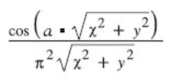
Maple actually operates both at the symbolic and numeric levels. If f(n) had not been defined before trying to evaluate it, Maple would return f(3), f(4), �f(10). This capability extends to differential equations and calculus including integration and differentiation. For example, you can enter an expression such as
The combined action of highlighting the expression and clicking the right mouse button brings up a list of operations that may be performed. Selecting differentiation results in
where the arrow indicates an operation has been performed.
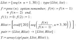
Returning to the evaluation of ?, to satisfy the golden mean, one side of a rectangle should be 1.618… times as long as the other. Mathematically, ?-1 = 1/?. This means that starting with a rectangle having its sides in the ratio of 1:?, if you remove the largest square possible, the remaining rectangle also will have its sides in the ratio of 1:? and so on. The following expressions evaluate and list successive ratios of adjacent Fibonacci numbers:
These entries closely follow a similar evaluation in Dr. Futschik�s paper. I wanted to print several successive quotients and their corresponding index values. Llist is the left-hand list of indices from 1 to 30, and Rlist is the right-hand list of quotients. The square brackets indicate a list. Maple rigorously enforces type checking so, for example, lists and arrays are distinctly different although one can be converted to the other explicitly.
Because the procedure was defined as f(n), the first value evaluated by the evalf(seq�) statement is f(3). Evalf is a Maple routine that numerically evaluates expressions and returns answers in floating point format with the number of digits specified in the [ ] option, in this case 20.
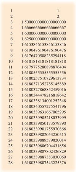
Two lists were developed so that they could be paired and printed as pairs. Pair is defined as an operator that associates members of the two lists. In the last statement, T is defined as the zipped array comprising the two lists Llist and Rlist. Because Rlist has only 28 entries, T is limited to 28 rows. The end result is displayed in Table 1 and shows that the f(n)/f(n-1) ratio converges to 1.6180339887 after only 28 iterations.
Table 1. Iterations of Fibonacci Number Ratios Converging to the Golden Mean
It is important to be rigorous in your language when describing how to use Maple and what it does. This can be difficult because ordinary English words have special meaning when used in a mathematical context. For example, although Table 1 looks like a table, in Maple�s terms it is not a table but rather a single-column array formed by zipping two separate single-column lists using the pair operator.
Fractals
One of the reasons I wanted to develop an expression for ? was to get experience working with recursive sequences. The more interesting challenge beyond Fibonacci numbers was to experiment with fractals. The following material is based on a discussion of Markus-Lyapunov fractals found while browsing mathematical websites.3
The development starts with the logistic formula, b(n+1)=r*b(n)*[1-b(n)]. Clearly, this is very different from the Fibonacci number series but will use similar types of Maple expressions. As the parameter r is varied, b behaves differently. For some values, b converges to a constant after a number of iterations n. For a larger r, b alternates between two values. And for yet larger r values, b appears to take on almost random values.
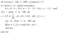
Arriving at this final nested do loop expression was not straightforward, but I learned a lot along the way. In Equa-tion 1 on page 14 that defined the Fibonacci series as a procedure with parameter n, the remember option was included. Maple remembers the results it has evaluated as an evaluation progresses. Especially for recursive functions, this is very important. For example, if previous values were not saved, each successive evaluation of f(n) would require evaluating all previous values for n-1, n-2�.
My initial attempts at evaluating the logistic formula were based on a similar procedure definition: b(n):= proc(n) option remember, b(n):= r*b(n-1)*[1-b(n-1)]. This worked well and appeared to be correct for different values of r and n. On closer examination, it was obvious that b(n) values were the same for different values of r. The remember feature was at work.
Because b(n) was only a function of n, once a particular value such as b(5) was evaluated and remembered, changing r made no difference to b(5). Including a forget statement caused b(n) to be reevaluated each time r changed. Although I could have included the forget function, I decided to redefine b as a procedure with both r and n as parameters to avoid the problem.
I also encountered the very basic difficulty of not being able to run a simple do loop in document mode. Perhaps I was not using the correct syntax, but the identical expressions ran correctly in the worksheet mode, so I completed the fractal exercise in the worksheet mode. Running and debugging nested do loops also required learning about Maple�s printlevel function.
Printlevel controls the amount and kind of output Maple returns when evaluating expressions. The default is print-level:= 1, which corresponds to top-level expressions. The printlevel associated with nested do loops increases with the depth of nesting. This means that unless you change the printlevel, no output will appear from an inner do loop: no, not even output from a print statement temporarily inserted to help debug the lack of output.
The array B basically is a square array with 100 columns corresponding to different r values. Each column has 101 rows, the first of which is the value of r, much as category labels are entered in Excel.
Based on the previously mentioned fractal article, r values between 2.5 and 4 were used because they give interesting results. The outer loop with column index i increments r from 2.5143 to 3.9285 in steps of 0.01428, storing successive values in B[1,i]. The inner loop with index m increments the array row address, taking into account the first row reserved for r values.
Once the array has been filled, the problem becomes one of plotting pairs of X-Y points to generate the fractal diagram. Maple doesn�t plot from an array; it plots values from lists. The obvious approach is to convert the array to a list, and there is a utility that will convert a 2-D array to a list of lists. This action would create an expression of the correct type , but I don�t know how to plot from a list of lists.
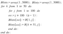
For example, there would be no way to specify X values as B[1,i], i=1..100. Rather than pursue this approach, I used a couple of do loops to fill two single-column arrays with X and corresponding Y values.
The inner j index serves two purposes. An address pointer is needed so that Blistx and Blisty can be filled, and the variable aa accomplishes that. The first value of r is written to the first, 101st, 201st�4,901st Blistx locations. The second value of r is written to the second, 102nd, 202nd�4,902nd locations and so on. Eventually, Blistx is filled with 50 contiguous ordered lists of the 100 values of r.
Blisty simultaneously is being filled with corresponding Y values from the last 50 iterations that originally filled the array B. To avoid plotting intermediate values before b(r,n) converged to a representative result, the first 50 iterations are skipped. The column index for the B array data written to Blistx and Blisty is always j, so the data is guaranteed to correspond to the correct value of r.
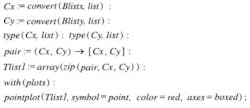
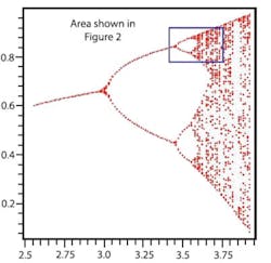
The next step is to convert the single-column arrays to lists. I found a separate variable was needed if I was going to effect the required type change. Just entering convert (Blistx,list) didn�t have the desired effect. Blistx remained an array. However, once I used the Cx and Cy lists and paired them as in the Fibonacci number example, the only thing left was to work with the pointplot function. Actually, this was the easiest part, and the plot shown in Figure 1 behaved as described in the Maple Help pages.
I made a lot of visits to the Help pages, generally coming away with a clue to what I needed to correct. On the other hand, I never found out how to edit the expressions I was entering. I could drag and drop some of them after entry, and changing a character was easy, but I simply could not make the entry cursor move to the beginning of the next line. In part, this was due to the auto-execution mode of operation in which Maple evaluates the expression(s) to the left of the cursor when you press the return key. I tried to use the many typesetting facilities and editing codes but without success. I was missing the basic understanding that seasoned Maple users have when it comes to manipulating equations.
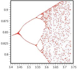
The logistic formula can be interpreted as describing an animal population. The variable r is called the fecundity factor, and as it increases from 2.5 toward 3.0, the population b also increases slowly but remains stable at a single value for any value of r in that range. Above about r = 3.0, the plot shows two distinct values for b, indicating an oscillation between plenty of food and a growing population and not enough food and a shrinking population.
Beyond about r = 3.45, there first are four stable states then rapidly many more until, for larger values of r, the plot appears to become chaotic. Nevertheless, there remain areas clear of points and areas where the points tend to group. Expanding the area to the right of r = 3.4 (Figure 2) reveals patterns very similar to the larger pattern in Figure 1, and further expanding each of these would have the same effect again. Replicating a pattern as the magnification is increased further and further is a characteristic of fractals.
To produce Figure 2, I changed the statement that incremented r to be r:= 3.4+i/300, resulting in a magnified X range. To achieve greater magnification in Y, I altered the pointplot expression to include a view option, view=[3.4..3.75, 0.78..0.92] where the first set of values represent the X-axis range and the second set the Y-axis range. New b(r,n) values were generated by rerunning the nested do loops.
Further Maple Impressions
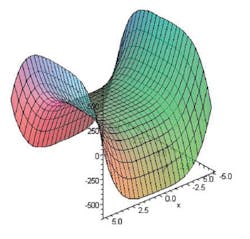
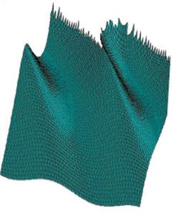
Much of the time used to prepare this article was spent learning to use Maple through the Fibonacci number and logistic formula examples. But, there are many new, easy-to-use aspects of Maple 10 as well, such as 3-D plots. After entering a formula, the combined actions of placing the cursor over the text and right clicking brings up a list of allowable operations. Plotting is one of these, and when selected, you have the option of using the new interactive Plot Builder routine.
Maple 10 also contains a Maplet Builder that helps you create graphical interfaces, task templates that are good starting points for solving more than 200 different tasks, and a handwriting recognition pallet: If you can�t find the symbol you need, sketch it, and Maple will provide a pretty version.
There are new functional packages that address statistics, statistical process control, and tolerances. You now can enter expressions together with their individual tolerances. In addition, Maple 10 handles units checking.
An important habit to get into when working with physical quantities is to include their units in calculations. Rather than simply remembering as you are entering a statement that one number is a mass and the next a force, include the units. Maple works with several consistent sets including MKS, FPS, CGS, atomic, SI, MTS, and ESU. Units checking is an easy way to find errors in equations.
The best advice for anyone needing a mathematical package is to try one before deciding to buy any. Make up a list of the typical kinds of problems you have to deal with, and see how easy it is to solve them with a given program. If the program is easy to use, what else can it do? How far into the future is it likely to be useful to you? How much can you afford to spend? Whatever your needs, if you decide to use Maple, you won�t quickly run out of capability.
Neither do you need to anticipate a long learning period. At the Maple Application Center, you will find more than 2,000 free applications, tutorials, and other resources. Maple Mastery I is a series of self-paced video lessons, another means of rapidly getting to grips with this powerful program.
Having become familiar with Maple 10, I can see where many of its basic math and plotting features will be helpful for developing future articles. For more specific needs, you can add capabilities from complementary Maplesoft and third-party products. Examples include fuzzy modeling and analysis, tools to integrate JDBC�/ODBC compliant databases, automated design of passive and active electronic filters, and signal processing via harmonic analysis.
References
1. Futschik, Dr. F., �An Algorithm to Approximate Pi,� Maple Worksheet, March 2005, www.maplesoft.com/applications/app_center_view.aspx?AID=1658&P=mr200503
2. The Golden Mean, http://goldennumber.net/history.htm
3. Markus-Lyapunov Fractals, http://perso.wanadoo.fr/charles.vassallo/en/lyap_art/lyapdoc.html
FOR MORE INFORMATION
on Maple 10
www.rsleads.com/508ee-209


