Essential Steps For Making High-Quality Electrical Measurements
Accurate measurements are central to virtually every scientific and engineering discipline, but measurement science tends to suffer for a couple of reasons. For one, it musters little attention in the undergraduate curriculum. Secondly, even for those engineers who received a thorough grounding in measurement fundamentals as undergraduates, it’s certainly possible—and forgivable—if they’ve forgotten some of the details.
When considering a measurement instrument for an application, the specification or datasheet is the first place to look for information on its performance and potential limitations in terms of results. However, datasheets sometimes may be difficult to interpret due to their specialized terminology. In addition, one can’t always determine if a piece of test equipment will meet the application’s requirements just by looking at its specifications. For example, the characteristics of the material or device under test may significantly affect measurement quality. The cabling, switching hardware, and the test fixture, if required, also could influence the test results.
The process of designing any test setup and characterizing its performance can be broken down into a number of steps. Creating such a flow greatly increases the chances of building a system that meets requirements and eliminates unpleasant and expensive surprises.
Table of Contents
-
Define The System’s RequiredMeasurement Performance
- Resolution
- Sensitivity
- Accuracy
- Repeatability
-
Select Equipment, Fixtures Based On Specs
- Accuracy
- Temperature coefficient
- Instrumentation error
- Sensitivity
- Timing
-
Build And Verify The Test System
- Lead resistance
- Thermoelectric EMFs in connections
- External interference
- Recheck System Performance
Define The System’s RequiredMeasurement Performance
To accomplish this task, one must understand some specialized measurement terminology:
-
Resolution: Resolution is the smallest portion of the signal that can be observed. It’s determined by the analog-to-digital converter (ADC) in the measurement device. There are several ways to characterize resolution—bits, digits, counts, etc. The more bits or digits, the greater the device’s resolution. Most benchtop instruments specify resolution in digits, such as a 6½-digit digital multimeter (DMM). Be aware that the “½ digit”terminology means that the most significant digit has less than a full range of 0 to 9. As a general rule, “½ digit”implies the most significant digit can have the values 0, 1, or 2.
-
Sensitivity:Sensitivity and accuracy, often considered synonymous, are actually quite different. Sensitivity refers to the smallest detectable change in the measurement, and is specified in units of the measured value (e.g., volts, ohms, amps, degrees, etc.). An instrument’s sensitivity is equal to its lowest range divided by the resolution. Therefore, the sensitivity of a 16-bit ADC based on a 2-V scale is 2 divided by 65536 or 30 µV. Instruments optimized for making highly sensitive measurements include nanovoltmeters, picoammeters, electrometers, and high-resolution DMMs.
-
Accuracy:Both absolute accuracy and relative accuracy must be considered. “Absolute accuracy”indicates the closeness of agreement between the result of a measurement and its true value, as traceable to an accepted national or international standard value. Devices are typically calibrated by comparing them to a known standard value (most countries have national standards that are kept in their own standards institute). Instrument drift is the ability of an instrument to retain its calibration over time. “Relative accuracy” is the extent to which a measurement accurately reflects the relationship between an “unknown” and a “reference” value.
The implications of these terms are demonstrated by the challenge of ensuring the absolute accuracy of a 100.00°C to ±0.01° temperature measurement versus measuring a change in temperature of 0.01°C. Measuring the change is far easier than ensuring absolute accuracy to this tolerance, and often, that’s all one needs for a particular application. For example, in product testing, it’s generally important to obtain accurate heat-rise measurements (e.g., in a power supply). However, it really doesn’t matter if it’s at exactly 25.00°C ambient.
- Repeatability:Thisrepresents the ability to measure the same input to the same value over and over again. Ideally, the repeatability of measurements should be better than the accuracy. If repeatability is high, and the sources of error are known and quantified, then high resolution and repeatable measurements often become acceptable for many applications. Such measurements may display high relative accuracy with low absolute accuracy.
Select Equipment, Fixtures Based On Specs
Interpreting a datasheet to determine relevant specifications to a system can be daunting. Some of the most important specs to evaluate include:
-
Accuracy:Many instrument vendors, such as Keithley, express their accuracy specifications in two parts: as a proportion of the value being measured; and a proportion of the scale that the measurement is on, for example: ± (gain error + offset error). This can be expressed as ± (% reading + % range) or ± (ppm of reading + ppm of range). Offset error is expressed as either a percentage of the range or ppm of the range. Gain error is expressed as either a percentage of the reading or ppm of the reading. Accuracy specs for high-quality measurement devices can be given for 24 hours, 90 days, one year, two years, or even five years from the time of last calibration. Basic accuracy specs often assume usage within 90 days of calibration.
-
Temperature coefficient:Accuracy specs are typically guaranteed within a specific temperature range. When carrying out measurements in an environment where temperatures fall outside of this range, it’s necessary to add a temperature-related error. This becomes especially difficult with widely varying ambient temperatures.
-
Instrumentation error:Some measurement errors result from the actual instrument. Instrument error or accuracy specifications always require two components: a proportion of the measured value, sometimes called gain error; and an offset value specified as a portion of full range.
-
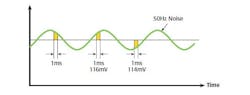
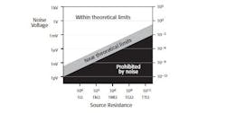
Sensitivity:Either noise or an instrument’s digital resolution may limit sensitivity, which is the smallest observable change detectable by the instrument. Often, an instrument’s noise level is specified as a peak-to-peak or RMS value, sometimes within a certain bandwidth. It’s important that the datasheet’s sensitivity figures meet your requirements. However, you also should consider the noise figures, because these will significantly affect low-level measurements.
-
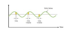
Timing.What’s the meaning behind a test setup’s “timing?” Obviously, an automated PC-controlled measurement setup allows for much quicker measurements than manual testing. This becomes particularly useful in a manufacturing environment, or in settings that require many measurements. However, it’s critical to ensure that measurements are taken when the equipment “settles,” because a tradeoff always occurs between the speed and quality of a measurement.
Rise time of an analog instrument (or analog output) is generally defined as the time necessary for the output to rise from 10% to 90% of the final value when the input signal rises instantaneously from zero to some fixed value. Rise time affects measurement accuracy when it’s of the same order of magnitude as the period of the measurement. If the length of time allowed before taking the reading equals the rise time, it will result in an error of approximately 10%. That’s because the signal only reaches 90% of its final value. To reduce the error, more time must be allowed. Reducing the error to 1% requires about two rise times, while reduction to 0.1% requires roughly three rise times (or nearly seven time constants).
Build And Verify The Test System
After choosing the appropriate instrument(s), cables, and fixtures, and establishing that the equipment’s specifications can meet the requirements, system assembly and performance verification become the next steps. It’s essential to check that each piece of test equipment is calibrated within its specified calibration period (usually one year).
If the instrument will be making voltage measurements, placing a short across the meter’s inputs will indicate any offset errors. This can be directly compared to the specifications from the datasheet. If the instrument will be used to measure current, then checking to see the current level with the ammeter open circuit will indicate offset current. Again, this can be directly compared to the specifications from the datasheet.
Next, include the system cabling and repeat the tests, followed by the test fixture and then the device under test (DUT), repeating the tests after each addition. If the system’s performance doesn’t meet the application’s requirements, taking a “one step at a time” approach should help identify the trouble spots.
After that, check the system timing to ensure sufficient delays exist to allow for settling time, and reassess it to make sure it satisfies the application’s speed goals. Insufficient delay times between measurements can often create accuracy and repeatability problems. In fact, this is among the most common sources of error in test systems, particularly when running the test at-speed produces a different result than when performing the test step by step or manually.
Although inductance can affect settling times, capacitance in the system is a more common problem. In a manual system, a delay of 0.25 to 0.5 seconds will seem to be instantaneous. In an automated test system, though, steps typically execute in a millisecond or less, and even the simplest systems may require delays of 5 to 10 ms after a change in stimulus to get accurate results.
Large systems with lots of cabling (and therefore, lots of cable capacitance), and/or those that measure high impedances (t= RC) may require even longer delays or special techniques such as guarding. Coaxial cable capacitance typically hovers around 30 pF per foot. The common solution is to provide sufficient delays—usually several milliseconds—in the measurement process to allow for settling. However, some applications may require even longer delays, which have led to more instruments including a programmable trigger delay.
The technique of guarding combats capacitance issues by reducing leakage errors and decreasing response time. It consists of a conductor driven by a low-impedance source surrounding the lead of a high-impedance signal. The guard voltage is kept at or near the potential of the signal voltage.
Although each system is unique, some error sources tend to be common in nature:
-
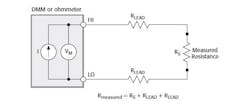
Lead resistance: Resistance of the test leads is a key factor in resistance measurements, especially at lower resistances. Consider, for example, the two-wire ohms method that’s used to determine resistance (Fig. 1a). A current source in the meter outputs a known and stable current, and the voltage drop is measured within the meter. This method works well if the resistance to be measured is much greater than the lead resistance.
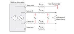
However, what if the resistance to be measured is much closer to the lead resistance or even less? In this case, using four-wire measurements will eliminate the problem (Fig. 1b). Now, the voltage drop is measured across the resistor, instead of across the resistor and leads. The voltmeter’s input resistance tends to be very high in comparison to the resistance to be measured; therefore, the lead resistances on the voltmeter path can be ignored. If, however, the resistance to be measured is exceptionally high, and approaching the voltmeter’s resistance, then it may require an electrometer or specialized meter with extremely high input resistance.
-
Thermoelectric EMFs in connection:In measurement systems, any connections made with dissimilar metals will produce a thermocouple. A thermocouple device, which essentially consists of two dissimilar metals, generates a voltage that varies with temperature (see the table). These qualities can be beneficial when monitoring temperature, but they will introduce unwanted voltages in standard test systems. As temperatures vary, so does the magnitude of the unwanted voltages. Even when connecting copper to copper, the composition of the two pieces of metal typically have enough differences to generate voltages.
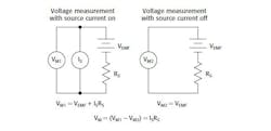
Sometimes, the magnitude of these errors is significant when compared to the value to be measured. The offset-compensated ohms technique, which is built into many instruments, can help eliminate the effect.
When enabled, the measurement cycle consists of two parts (Fig. 2). The first part measures the voltage with stimulus current switched on, and the second part measures the voltage with the stimulus current switched off. Subtracting the latter from the former will subtract out the errors due to thermoelectric EMFs. Consequently, it effectively eliminates accuracy issues caused by temperature drift.
Even after the test setup assembly and verification, it’s important to recheck the system’s performance on a regular basis. An instrument’s accuracy will vary over time due to component drift. Thus, instrumentation should be calibrated regularly. For a more in-depth exploration of the topics discussed in this article, check out Keithley’s archived online seminar, “Understanding the Basics of Electrical Measurements.”
Derek MacLachlan, applications engineer at Keithley Instruments, holds a degree in electronic and software engineering from the University of Glasgow in the United Kingdom. Contact email is [email protected].
About the Author
Comment About the Article
To join the conversation, and become an exclusive member of Electronic Design, create an account today!

Leaders relevant to this article: