Making Accurate Bandwidth Measurements
Everybody already knows what bandwidth is and how it is measured. The problem is the definition: bandwidth is defined and measured in remarkably different ways by different people.
In the basic scheme used to determine bandwidth, you apply a leveled sine source to the device under test and measure the output signal. As the frequency increases, the bandwidth is the point where the response first drops to 3 dB below the low-frequency reference value.
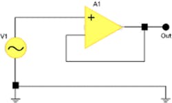
As an example of this measurement method, Figure 1 (see below) shows a constant-amplitude sine wave being applied to a buffer amplifier. For this DC-to-band-limit case, we can consider the following:
- A measuring instrument such as an AC voltmeter, a spectrum analyzer, or an analog-to-digital converter (ADC).
- A source such as a leveled sine generator or an AC calibrator.
- A pass-thru element such as an amplifier or a filter.

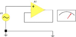
The Simple Measuring Instrument
The measuring instrument is shown as a moving coil meter in Figure 2 (see below), but this is just a representation of a generic instrument. Using the simple method, we measure the output signal at some low reference frequency. Then we turn up the generator frequency until the indication drops by 3 dB. Of course, a flat signal-generator source has been assumed, and up to 100 kHz, this is a very reasonable assumption.
Figure 2. Schematic of Simple Measurement Circuit With Meter
The measuring instrument is assumed to have a relatively high input impedance: 1 MW in parallel with not more than 100 pF. The leveled sine source should have less than 50-W output impedance. This combination gives a theoretical flatness error of less than 5 ppm, which is swamped by other error sources.
The leveled source at low frequencies ordinarily would be an AC calibrator, and it usually would have a four-wire force-sense arrangement. As a result, the 100 pF of lead capacitance and the 100 pF of load capacitance would not present a direct loading error but some lesser error due to the finite closed-loop output impedance.
In general, these errors are negligible when measuring low-frequency, 3-dB bandwidths. The measurement uncertainty of the voltage impressed on the input terminals of the AC meter could be closer to the 100-ppm level than the gross -29% that the meter will be reading at its -3-dB point.
In this application, there is no need to worry about the calibrator. It certainly will have noise and harmonic distortion on its outputs, but in terms of the bandwidth, these are not an issue. However, if we had a criterion of a 0.1% deviation of response on the meter rather than 29%, then harmonic distortion on the calibrator would be of considerably greater importance. Even more important would be the exact nature of the measuring instrument.
What Is Being Measured?
We are making an AC rms measurement, and there are many ways to display the reading:
- Half-cycle mean responding, rms calibrated.
- Peak responding, rms calibrated.
- Peak to peak responding, rms calibrated.
- rms responding, rms calibrated.
The classifications get better as you go down the list. The last type—a true rms instrument—is optimal. Often you end up with one of the lesser categories.
If you want to calibrate your meter accurately, then verify your calibrator with the same methodology as the meter you are calibrating. In other words, use a peak-to-peak method to verify a calibrator when it is being used to calibrate a peak-to-peak responding instrument. If not, then allow for the harmonics and the noise.
Notice that when measuring bandwidth, the harmonics are progressively further outside of the meter passband, so as the order increases, they have less effect. However, if you are looking at the 1% flatness point of the meter, then the harmonics certainly are not outside the meter passband, and they can have an alarmingly large effect.
Suppose the calibrator has -40-dB of second-harmonic distortion at the frequency of interest. This distortion is 1% and directly affects the meter reading. A 1% second-harmonic distortion into a peak-sensing meter will give ±1% uncertainty. A 1% second-harmonic distortion into a peak-to-peak sensing meter will make it read 50-ppm high ±100 ppm (-50 ppm to +150 ppm). However, 1% second-harmonic distortion into an rms sensing meter will give no error at all if, as is usual, the calibrator was calibrated with an rms responding transfer standard.
Finally, consider an ADC in this context. Normally, ADC bandwidth would be specified in terms of a reduction of the fundamental signal by 3 dB. In other words, apply a sinusoidal input, convert the data to digital form, do a fast Fourier transform (FFT) of the data, and then look at the amplitude of the fundamental. If the ADC distorts the signal near its band limit, as they usually do, then the peak-to-peak 3-dB point of the data will not coincide with the fundamental 3-dB point.
A Higher Frequency Meter
Obviously, this method breaks down at UHF frequencies (>300 MHz) where the short lengths of cable from the T-piece no longer can be neglected. We formally could refer to this method as an external reference plane calibration. Informally, we are forcing the input terminals with a voltage, so we could say it was a terminal voltage calibration, just like the low-frequency method previously described.
This is a good method of calibrating high-input impedance devices such as RF probes because the probe will give a correct indication of the signal at the probe tip. The probe may load and reduce the signal, but the probe still would be reading the voltage at its tip. In fact, the loading effect of the probe then could be established by seeing how much some other output measurement was changed, first with and then without the probe.
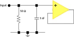
This, however, is not a good method for calibrating devices with a low-input impedance, especially if the input impedance is variable with frequency. Let’s suppose the meter has an input impedance of 1 MW//20 pF. At a frequency of 10 MHz, the input impedance effectively is a 796-W reactive load. This may well have a significant loading effect on the measured signal. At 100 MHz, continuing with this simple model, the impedance of the meter is 79.6 W.
To make the meter have a flat response up to very high frequencies, provide a 50-W input. In this way, the coax cable, which is chosen to have a characteristic impedance of 50 W, does not change the input impedance of the meter (with this simple model at least).
The input impedance of the meter is specified in terms of the voltage standing wave ratio (VSWR) and related to the reflection coefficient r by:
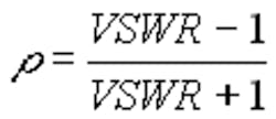
This gives the magnitude of the input reflection coefficient. For every reading taken in a pure 50-W system, you need to factor in an uncertainty contribution due to the reflection coefficient. The reading must be multiplied by 1± r to account for the uncertainty.
If the VSWR is 1.5, the reflection coefficient magnitude is 0.2 or a ±20% uncertainty. For this reason, the terminal voltage method is useful only for devices with input VSWR values around the 1.05 level.
However, a manufacturer is entitled to sell its product with a bandwidth measured by the terminal-voltage method. The customer must ask nagging questions such as:
- How is the bandwidth specified?
- How is the bandwidth verified?
- What is the input VSWR?
UHF Calibration
The calibration method used in Figure 3 is the reason why the uncertainty of the measurement was so large. If the meter was calibrated in a true 50-W system, then there would be no additional measurement uncertainty when it was used in a true 50-W system. A smaller correction accounts for the fact that the measured system, and indeed the calibration system, will not be ideal, but this is a considerably smaller error.
The second method is known as incident voltage calibration and should be used to calibrate RF voltmeters, scopes, and spectrum analyzers. The term 1± r is included in the calibration constants for the meter, and it is up to the manufacturer to get the meter to read correctly with this connection method.
The error term that is needed is called the mismatch uncertainty 1± rMrS , also known as the multiple mismatch uncertainty factor. This has reflection coefficient (magnitude) terms from both the source and the meter, but the multiplication reduces the overall value. For example, if both the meter and the source have reflection coefficient magnitudes of 0.2, the mismatch uncertainty is ±4%.
The terminal voltage calibration method also uses the mismatch uncertainty term for nonideal sources, so it has two uncertainty terms. The general formula for the terminal voltage is:
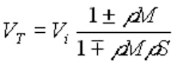
Notice that the magnitudes always are taken in their worst possible polarities to give the limits of the uncertainty.
Which Bandwidth?
Depending on whether you mean incident- or terminal-voltage bandwidth, the term bandwidth applied to a non-50-W board-level pass-thru type of component is remarkably uncertain. Actually, by suitable choice of external components, it is easy to make the overall bandwidth measurement change by a factor of two or more.
VSWR is another ambiguous area. When specified, it usually is given as less than some value. This does not mean that it monotonically decreases with frequency. If the VSWR spec is less than 1.5:1, you will find situations where the VSWR increases to this value at some lower frequency, then heads back down. Consequently, it is possible to get a lower peak VSWR by compensating the input impedance.
Similarly, it is possible to get considerably more bandwidth from a 50-W component by deliberately making the VSWR worse. For example, if an inductor is put in series with the 50-W input termination resistance, the terminal voltage will be peaked, and this can compensate for bandwidth rolloff in subsequent stages.
By the same token, a designer can get more bandwidth in an individual amplifier stage by tuning the input and output reflection coefficients. This is because the maximum power transfer is achieved by conjugate matching the load and the source. If the source has an impedance of Z = R + jX, the conjugate match condition requires the load to have an impedance of Z* = R – jX. The reactive components cancel, which you could consider as a resonance condition.
Even though the input resistance of a UHF-capable device at DC is 50 W ±1%, it doesn’t mean that the resistive part of the input impedance remains at 50 W over all frequencies and that the nonunity VSWR results from a reactive component.
Regardless of the resistance at DC, a 50-W device with a VSWR of 2 can have the resistive part of its input impedance looking like 25 W or 100 W or anything in between. The fact that the DC resistance is correct is not relevant.
Generators
Usually the flatness of a signal generator is specified rather than the 3-dB bandwidth. Leveled sine generators are available with flatness specifications of a few percent, but you cannot use the manufacturer’s flatness spec on its own. The actual flatness you get into an RF load must take the mismatch uncertainty into account as well as the specified flatness of the generator.
Having consulted with experts at the National Institute of Standards and Technology and the National Physical Laboratory, if you want to measure the source reflection coefficient of your leveled sine generator, then probably you are better off not using a leveled sine source. The experts use 2-resistor power splitters or directional couplers to make hybrid sources that emulate leveled sine generators but have well-defined, low-output reflection coefficients. Directly measuring the output reflection coefficient of a leveled sine source is difficult and uncertain.
Another technique is to attenuate the sine source with a good low-VSWR 10-dB attenuator. This will guarantee that the generator has an effective reflection coefficient magnitude below 0.1.
The rolloff characteristic of a meter also contributes to measurement uncertainty by as much as tens of percents. The problem is one of converting an amplitude uncertainty to a bandwidth uncertainty.
In an ideal single-pole meter, a ±1% voltage uncertainty at the 3-dB point would translate to a ±2% uncertainty in the bandwidth. In a real system, you would have to plot the rolloff characteristic to ascertain the slope of the rolloff in the 3-dB region. Under these conditions and above 200 MHz, the bandwidth reading on one meter could read tens to hundreds of megahertz differently compared to another.
Conclusion
RF measurements, and bandwidth measurements in particular, have specific terms and techniques that trip up the unwary at every turn. At DC, you can take the accuracy figures of calibrators and signal generators at face value. However, when dealing with 50-W systems, you need to understand the magnitude of the uncertainty of your measurement. Armed with the mismatch uncertainty formula and the definitions of incident voltage compared to terminal voltage, you should have a better chance of quantifying such measurement uncertainties.
About the Author
Leslie Green, CEng MIEE, is a senior principal engineer at Gould-Nicolet Technologies and a graduate of Imperial College with a B.Sc. He has 20 years of experience in developing test and measurement equipment, initially at Datron. For the last 14 years, Mr. Green has been designing oscilloscopes for Gould-Nicolet. Gould-Nicolet Technologies, 2-8 Roebuck Rd., Hainault, Ilford, Essex IG6 3UE, U.K., 011 44 181 500 1000.
Return to EE Home Page
Published by EE-Evaluation Engineering
All contents © 2001 Nelson Publishing Inc.
No reprint, distribution, or reuse in any medium is permitted
without the express written consent of the publisher.
February 2001
About the Author
Comment About the Article
To join the conversation, and become an exclusive member of Electronic Design, create an account today!

Leaders relevant to this article: