This article is part of the Analog Series: Back to Basics: Impedance Matching
Impedance matching is one of those design processes that you use to make circuits and equipment work properly. It’s a process you probably learned in college, or not. The basic rule is simple:
To achieve maximum power transfer, the load impedance should be equal to the source impedance, or some variation thereof.
Of course, there’s more to it than first meets the eye. If you’re an RF engineer, you probably use this process all of the time. Other engineers never seem to need it. If you’re writing code for an embedded processor and interfacing it to some external circuits, you probably couldn’t care less.
A while back, I wrote a three-part series of articles on impedance matching that sums up the basic processes for those needing a refresher or just learning it for the first time. After getting such a great response to this series, we decided to update the current series. All three parts have been revised to include new material and useful reader feedback.
If you missed this series of tutorials, you can now find them as part of this series. Here’s a quickie summary of the content to help you zero in on your needs and interests.
Part 1 states the maximum power transfer theorem and goes on to illustrate its importance. Following that, some basic impedance matching circuit and methods are described. A discussion of matching audio amps to speakers concludes that not all things must be matched.
An important feature of Part 1 talks about transmission lines and how many things are interconnected with coax. It’s essential to match impedances when using transmission lines, as the consequence of not matching produces high standing wave ratio (SWR) and significant power loss. Coax matching methods are provided. This part wraps up with a section on transformer impedance matching.
Part 2 focuses on impedance matching with L-networks. L-networks are the mainstay of RF impedance matching. They’re simple and remarkably effective. Techniques for designing these networks are given with multiple examples.
Part 3 shows how to design pi and T-networks. These are derived from the L-network and provide a way to match a wider range of impedances with the ability of controlling Q. They’re particularly useful tools in RF circuit design. This part also covers automatic matching with tunable networks. These have been widely adopted in smartphones to keep the antennas tuned for maximum output and input regardless of physical orientation and condition.
There were a few items I was not able to cover in the initial series, so I’ll be adding two more parts.
Part 4 delves into automatic Z matching. It discusses how to get your antenna to tune itself for maximum effect.
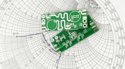
The series concludes with Part 5, which shows how you can use the Smith chart to do your impedance matching. Luckily, some software is available to simplify and facilitate this process.


