Part One: Linear Superposition Speeds Thermal Modeling
Linear superposition, as its name implies, is associated with linear systems. In your core undergraduate electrical circuits class, you learned that networks comprising only resistors, capacitors and inductors fall into this category. But an analogy can be made with thermal systems, which typically consist of only resistances and capacitances, so they, too, can look like linear systems. There are certainly situations where thermal resistances — and sometimes even capacitances — don't act very constant. However, the basic equations describing the behavior of elements are written as if they were constant, and this assumption provides a convenient starting point for thermal analysis.
Thermal linear superposition says that if you turn on each component in the system by itself, and measure its effect on all the other components, then when you turn them all on at the same time, you can simply add up the individual effects each had alone, and you'll get the correct overall effect.
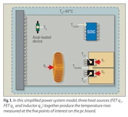
Consider a simplified power-supply system as in Fig. 1, where we'll suppose that there are only three significant heat sources: two FETs (q1 and q2) and a coil (q3). We're interested in five temperatures: the two FETs (TJ1 and TJ2), the case of the axial-leaded device (TX), the ground pin on the small-outline IC (TL1) and the board location midway between the FETs (TB). This system may be expressed mathematically through the following matrix equation:
Eq. 1 is actually just a shorthand notation for five separate equations, relating the five temperatures of interest (a temperature vector consisting of ΔTJ1… ΔTB) to the three identified heat sources (a power vector consisting of q1, q2 and q3), through the array of 15 coefficient values in the middle (a theta matrix). If we were to write out these equations separately, the second equation, describing the junction temperature of FET#2, for instance, would be:
where ΔTJ2 is the rise in TJ2 for the given power vector and theta coefficients, Ψࡋ is the thermal interaction coefficient giving the temperature rise at FET#2 due to heat at FET#1 (q1), θJ2A is the thermal resistance from junction to ambient of FET#2, and Ψࡋ is the thermal interaction coefficient giving the temperature rise at FET#2 due to heat at the coil (q3).
There are a couple of important points to note. First, Eq. 2 is linear as long as the three coefficients multiplying the power dissipations are constant. This implies that if every heat source doubles, the temperature rise will double. Second, Eq. 2 is a direct expression of the idea of linear superposition. It says the temperature rise at junction 2 is a linear combination of three individual terms, each of which is the temperature rise that junction 2 would experience if that particular heat source were the only heat source.
From Eq. 2, you can also see that the effective θJA for device 2 isn't defined by its own properties alone. Note that we've used the term θJ2A as the coefficient for the power dissipated by device 2, because if device 2 was the only heat source present, we'd have the basic definition of its θJA expressed in the simpler equation:
If you solve Eq. 2 for the effective θJA as experienced by device 2 in the complete interacting system, you find:
Thus, what device 2 sees in isolation, θJ2A, is not necessarily anything like what it sees when other components are present and contributing power. Obviously, the magnitudes of the interaction terms (Ψ, Ψ) figure prominently. More significantly, observe that as device 2 power approaches zero, there is no upper limit for the effective value of its thermal resistance. This is why some component manufacturers are smart enough to refuse to put θJA in their absolute maximum ratings tables.
In Eq. 1, all the temperature vector elements are indicated as ΔTs, because in the simplest thermal systems there is a common thermal ambient (TA) to which all temperatures can be referenced. (All heat is flowing to the same ultimate thermal ground.) However, if you want to explicitly refer to ambient, you could have written Eq. 1 like this:
Spreadsheet Math
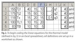
Let's jump right in to show how easy it is to code up a set of linear equations in Microsoft Excel. We'll use the Eq. 5 version of our model as the example, because this provides a basis for thermal modeling for cases where there's a whole set of reference temperatures rather than just a single value. Fig. 2 shows how you might set up your cell definitions in an Excel worksheet.
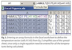
Given specific values for the theta matrix (cells D1:F5), power vector (cells H1:H3) and ambient (cells K1:K5), the values in column A arise from a simple formula typed into Excel, which appears in all five of the temperature cells (A1:A5), as shown in Fig. 3.
The squiggly braces around the formula up in the formula bar are not typed in; Excel inserts them automatically when you use Ctrl-Shift-Enter to input the formula after you type it in (with all five cells selected at once). They indicate that the formula is, in Excel terms, an array formula; correspondingly, the formula refers to entire ranges (arrays) of cells as its arguments. The MMULT, for matrix multiply, function is built into Excel and performs the magic of doing exactly what we've expressed in Eq. 5, all at once. So you don't have to code five separate equations as you might have thought from Eq. 2, and it should be clear that as far as Excel goes, you could just as easily have 12 heat sources and 17 temperature locations; you'd still have a single array formula, and you'd create it in one easy step.
The Theta Matrix
So, where do we get the values that go into the theta matrix? We're going to assume that there's no way you're going to find datasheet values for most of the numbers in the matrix. (Even if you had curves showing θJA versus copper spreader area and airflow for the FETs, and you believed they were a good fit to your board, all those interactions between devices are totally beyond anything you'll find from a component manufacturer.) If you're handy in the lab, this is the most direct approach to take:
Step 1: Power up FET#1 without putting power anywhere else, and measure all five temperatures of interest. Be sure that you also establish any other significant boundary conditions. It will not do to make a several measurements in still air with the box wide open, when you are ultimately trying to predict the performance of your system with a big fan pushing air through your box.
Step 2: Compute the five coefficients of the first column of the theta matrix from those measurements, namely:
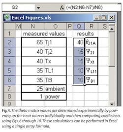
Note that all five of these values are computed using the actual power you supplied to FET#1 during this characterization experiment, and they're also all based on whatever ambient happened to be in the lab at the time. Fig. 4 illustrates how easily all five of these calculations can be done using a single Excel array formula.
Step 3: Turn off FET#1 and turn on FET#2. Measure all five temperatures, and compute the second column of the theta matrix in a similar way.
Step 4: Turn off FET#2 and put some power in the coil. Calculate the third and final column of the theta matrix.
Once you've got the theta matrix, you can use this model to predict temperatures at all your locations of interest, at any other power distribution you choose: Just plug different values into column H, of the Excel model shown in Fig. 2, and new predictions appear in column A.
Contingencies
Of course, the real world isn't always so cooperative, and the experimental methodology I've outlined may cause you some trouble. So let's talk about some alternatives.
First, what if you can't put enough dc power into the coil to heat up anything? After all, these are dc measurements I'm talking about, and the coil's resistance is pretty low. Maybe you can't put significant power into the coil without running the power supply at frequency, under load. But obviously if you do that, you're also dissipating power in the FETs, and the premise that you're only powering up one component at a time falls apart.
Here's one choice. Temporarily replace the coil with something that can dissipate a lot of dc heat — maybe just a 1-W axial-leaded resistor. The board doesn't really care what the heat source at the coil's location looks like, especially if you can send the heat into the same footprint. Since we don't care about the coil temperature itself, it really doesn't have to be a coil that puts the heat into the board at the coil's location.
Second, this does not have to be done experimentally. It can be done just as easily, sometimes more easily, through a simulation. A thermal simulation solves some problems we've alluded to: It's really easy to turn on the heat sources independently, and you can put as much heat into a coil as you want. Just follow the method outlined previously to generate your theta matrix, using the simulator as your lab.
Third, you don't have to power up everything completely independently. All you need are linearly independent power vectors to stimulate your system. So, if you can at least partially shift the power distribution from one device to another, then you can modify the data-reduction technique to solve for the theta matrix coefficients as if they were the 15 unknowns in a set of 15 equations.
For instance, we've got five temperature locations to worry about, but each location depends on its own unique set of three theta-matrix coefficients. Consider the board temperature. You've made a series of measurements with three different power vectors. Those measurements, indicated by the hyphenated subscripts, represent three equations in the three unknown coefficients:
Or in matrix form:
Which is to say you can solve for the unknowns — the original coefficients — by inverting the matrix of power values:
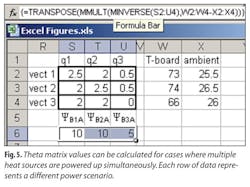
Again, Excel makes this so easy that you almost don't even have to know from where the math comes. Fig. 5 shows how you might lay out this data-reduction problem. In this example, each row of data represents one power scenario, where we allow that the lab's ambient temperature drifts around between measurements. Here, you see two more of Excel's matrix-manipulating functions in action: MINVERSE, for matrix inverse, which does what you might expect, and TRANSPOSE, which turns a column vector into a row vector, or vice versa. If you compare the output results (10,10,5) of this data reduction example, with the fifth row of the original theta matrix in Fig. 2, you'll realize that I didn't choose my input values for the board and ambient temperatures by accident.
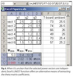
Speaking of matrix inversions, here's where the idea of linearly independent power vectors comes in. If the power vectors aren't linearly independent, then the power matrix will be singular and the inversion process will fail. If you're not sure you've created an obviously independent set of power vectors (and maybe even if you are), it's nice to make more measurements than you need — in effect, get more equations than you have unknowns for. You then use a different Excel approach to extract your model. Fig. 6 shows how to manage six power-vector scenarios, each with its own board and ambient temperature measurement, and use Excel's LINEST function to get the three coefficients we're after. LINEST performs a least-squares linear regression on a set of multiple, independent linear variables, as in y=m1x1 + m2x2 + m3x3 + b.
A couple of points regarding LINEST. First, observe that the third argument on the formula bar is zero; that forces LINEST to use a zero-intercept. After all, physically speaking, we know that if all power sources are turned off, all temperature rises must be zero. This intercept would have appeared in cell D10 in this layout, but as you can see, a zero was returned. LINEST also returns statistics on the coefficients (and the intercept, if used), which appear directly below each value (in row 11 of this example). Yet one additional statistic of interest (marked in red) is returned in cell A12, the infamous “r-squared” correlation coefficient; if the fit was perfect, this value would be exactly unity. You can see that my experimental data was pretty linear in this example. Finally, for reasons that remain obscure, LINEST returns the coefficients in the reverse order with respect to the input data. In other words, as you see in Fig. 6, q1, q2 and q3 appear from left to right in the input table (cells B2:D7), yet the three coefficients appear from right to left (as shown in cells A10:C10).
Note that the simultaneous power approaches build up the theta matrix row by row, rather than column by column as in the independent power method.
What if Nonlinearities Are Big?
If your system has significant nonlinearities (which could show up, for instance, as bad statistics in the LINEST analysis), most of the preceding techniques can still be applied, with a small modification. What we do is linearize the system behavior around a chosen operating point. Here's how:
First, choose a nominal operating point you think is close to where you're going to want to create predictions. Test, or simulate, your system at that point, and record all the power levels and temperature values you used to create it.
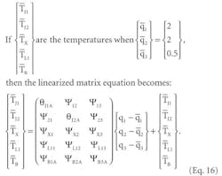
Now, systematically perturb your power vector from that operating point. For example, take each heat source in turn, and bump its value up (or down) a measurable amount from the nominal point, holding all the others constant. For each variation, record power levels and resulting temperatures. Your theta matrix will now be a set of coefficients that predict temperatures as small perturbations from the nominal values. In other words:
Eq. 5 can be thought of as a special case of Eq. 16, where the nominal power dissipations are identically zero and the nominal temperatures are ambient. The practical difference between a linearized nonlinear system and the ideal, perfectly linear system is the addition of one more measurement. If the system is nonlinear, the farther you move the actual operating point from the nominal operating point, the less accurate the theta matrix becomes.
With modest effort, you can construct a linear superposition model of your system before you know your final power distribution, and without later rerunning experiments or detailed simulations, you can predict critical system temperatures over a range of actual operating points.
