Understanding Your Signal Analyzer’s “Dynamic Range”


Dynamic Range DefinitionMost RF signal analyzer experts would agree with the following definition for dynamic range of an RF signal or spectrum analyzer.
Signal analyzer dynamic range is the maximum power ratio (in dB) between a high power signal and low power signal that are present at the input of the signal analyzer – such that both signals can be discerned and measured at the same time or in the same display.
While the above definition might sound simple enough, the fact is that instrument characteristic such as noise floor, resolution bandwidth, and linearity each affect one’s ability to discern a low power signal in the presence of a high power signal. Moreover, for most of these characteristics, their impact on one’s ability to discern a low power signal varies according to the signal power that is present at the front end of the signal analyzer.
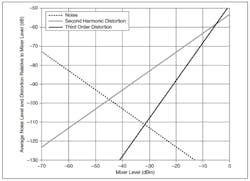
While I generally try to avoid using the words “dynamic range” whenever possible to avoid confusion, it’s certainly worth explaining what we commonly refer to as the “dynamic range chart” of an RF signal analyzer – arguably one of its most important specifications. Because instrument characteristics such as noise floor and linearity are power level dependent, the dynamic range chart is meant to characterize each of these as a function of the mixer level of the instrument - shown in Figure 1.
Mixer level = Input signal level – Attenuation
Mixer level = -20 dBm – 10 dB = -30 dBm
Given the dynamic range chart shown in Figure 1, it’s pretty easy to optimize an instrument for either noise floor or linearity (or a little of both) simply be setting its input attenuation. For example, when measuring adjacent channel power (ACP) on a modulated signal, the ideal mixer level is usually right at the intersection point of the noise floor and the third order distortion trace. The optimal setting for third order distortion measurements is similar, because this measurement involves discerning a relatively low power third order distortion tone in the presence of a much larger fundamental tone. Of course, it’s important to note that the “noise floor” trace in Figure 1 represents noise in a 1 Hz bandwidth. Thus, measuring IM3 levels higher than 100 dB or better requires extremely narrow resolution bandwidths, significant averaging, and a good deal of patience.

Because the dynamic range chart usually refers only to the downconverter portion of an RF signal analyzer, it’s important to understand the instrument’s architecture for best results. At the end of the downconverter is a narrowband intermediate frequency (IF) filter leading into an analog to digital converter (ADC). While it’s difficult to represent the effects of the IF filter and ADC on instrument performance in the same char, it’s worth knowing how these elements affect one’s ability to perform a top-notch measurement. Below, are a few tips that I’ve learned along the way.Most instruments employ a “headroom” of anywhere from 6 dB to 10 dB. The headroom represents the IF power ratio (in dB) between a nominal IF power level and “full scale” of the ADC. When making measurements on a signal with a relatively low peak-to-average ratio (PAPR), one can usually decrease the attenuation level of the analyzer (lower the reference level) by a few dB without clipping the ADC. This is especially important when measuring error vector magnitude on narrowband or OFDM modulated signals where the EVM floor of the instrument is often dominated by the noise floor. In most cases, the instrument will usually yield the best EVM performance right at the clipping level of the ADC.
The bandwidth of the signal analyzer’s last IF filter can significantly affect IM3 or ACP measurements. When making an IM3 measurement, be sure to set a narrow IF filter bandwidth (also called high dynamic range mode) and make sure that the stimulus uses a tone spacing that is wider than the IF filter bandwidth. This approach ensures that the signal analyzer’s ADC will never “see” a fundamental tone and a third order distortion product simultaneously – improving the IM3 floor of the instrument.
Finally, don’t be afraid to filter out the fundamental tone when making spurs or harmonics measurement. As we observed in Figure 1, even an out-of-band high power signal will still be present at the first mixer of an RF signal analyzer. In order to ensure that 2nd or 3rd harmonics of high power out-of-band signals do not affect a measurement, it’s often necessary to filter them out with a pre-selection filter. This filter can either be tunable (like a YIG tunable filter) or fixed-frequency – so long as the fundamental tone in the stop band of the filter. Conclusion
If there are two things I could leave you with, it would be to: 1) avoid using the term “dynamic range” unless you really mean to say it, and 2) make sure you understand the architecture of your instrument. As I mentioned in the beginning, I’ve seen enough people misuse the term dynamic range over the years that I think it’s better to be more specific on whatever characteristic you are describing. And of course, we’ve seen how a basic knowledge of RF signal analyzer’s architecture can lead to simple optimizations such as choosing the best reference level or IF filter bandwidth.Do you have any tips on how to get more out of an RF signal analyzer?
About the Author
David Hall
Head of Semiconductor Marketing
David A. Hall is the head of semiconductor marketing at NI and is responsible for developing and executing go-to-market plans for the semiconductor industry. His job functions include managing the semiconductor test business, identifying industry trends, and educating customers on best semiconductor test practices. Hall’s areas of expertise include ATE architectures, RF measurement techniques, digital signal processing, and best measurement practices for mobile and wireless connectivity devices.
With nearly 15 years of experience at NI, Hall has served in multiple roles throughout his career including applications engineering, product management, and product marketing for automated test and RF instruments. He has also held management positions in product marketing, which focused on employee development and meeting business results across products and application areas. Hall is a known expert on subjects such as 5G, the Internet of Things (IoT), autonomous vehicles, and software-defined instrumentation. He holds a Bachelor’s with honors in computer engineering from Penn State University.
Comment About the Article
To join the conversation, and become an exclusive member of Electronic Design, create an account today!

Leaders relevant to this article: