
So...Analog Computing Hits a Bump in the Road and All THAT (Part 2)
What You'll Learn
-
How to write out your own equations for a physical system like an automobile suspension.
-
How to transform those equations into a patch schematic to run an Analog Computer simulation.
-
Custom circuits can be built to solve specific problems, but they’re labor-intensive for solving multiple problems.
-
Bob Pease cheated and used a differentiator in his Analog Computer. He knew from experience what he could get away with and how to mitigate its dangers—and did.
- The world's first documented Programmable Analog Laptop Computer THAT is revealed in this blog and is suitable for STEM education.
Bob did it with parts
Anabrid uses patchcords
Difference is same
An automobile suspension is the classical 2nd-order system taught in undergraduate engineering schools—in my case, it was in our Dynamics class. After describing the relationships of mass, spring, and damper (or “dashpot”) in terms of displacement y, speed y′, and acceleration y′′, in calculus, we went off and wrote programs in Canadian Fortran (WATFIV...WATerloo (the University that wrote it), and “FIV” being the next generation of WAT-FOR (clearly their witty software naming didn’t age very well). We then took to the card punch and stood in line at the card reader, which jammed and ate a card now and then, to run the program on the school’s IBM 360 Mainframe.1
Some of you may have already downloaded the user guide for the THAT Analog Computer, described in my last blog. From the user guide, Section 9.2 on page 16, we have the diagram of an automobile suspension system (Fig. 1).

The car body and its occupants are represented by the mass block, which is suspended (hence “suspension”) on a spring that connects it to the ground (the tire/wheel is assumed for simplicity to be a solid object in this simplistic model, though with THAT, we certainly could add the “unsprung” mass of the wheel, hub, tire, etc., as well as a spring and a damper to model the tire’s compliance) with a shock absorber (aka “damper” or “dashpot”).
We can construct a FBD (Free Body Diagram — how I remember this term after almost 50 years is beyond me because I haven’t done an FBD since my university days) where all forces must be in equilibrium if the car is just sitting there; i.e., no net force results from the system. Therefore, the force of the Mass (Fm) must equal the forces of the damper (Fd) and of the spring (Fs):
Fm + Fd + Fs = 0
May the Forces be With You
We know that the force on a mass (m) is given by Newton’s 2nd Law of Motion:
Fm = ma, where a is acceleration
We also know that the force by a spring with spring constant k is given by Hooke’s Law as:
Fs = ky, where y is vertical distance or displacement
And the force in a damper with a damping coefficient d is given by Nobody’s Law (why is that?) as:
Fd = dv, where v is the vertical speed
About Your Car’s Differential...
Recall that speed v is the first derivative of position y′ and that acceleration a is the second derivative of position y′′ (with apologies for the lame Lagrange’s notation with apostrophes because Newton’s notation of derivatives is impossible on Electronic Design’s typesetter system. It’s barely capable of technical, scientific, and engineering scrawl beyond what the bunch of monks in the back room of Microsoft can do with their type sets. Now I know why Bob Pease was missing the equations in his blog on automobile suspension Analog Computing, here).
So, the differential equations are written as follows:
Fm = my′′
Fd = dy′
Fs = ky
Fm + Fd + Fs = 0 then becomes, by substitution:
my′′ + dy′ + ky = 0
And rearranging to solve for the highest derivative becomes:
my′′ = - ( dy′ + ky )
or
y′′ = - ( dy′ + ky )/m
Which is the form I have to leave it in because of the lame editing software created by a bunch of y′′′s at Microsoft.
Then THAT Rabbit Comes Out of the Hat
All of this math and physics stuff pretty much tracks with what’s in THAT’s Section 9.2 writeup. That’s good, because the equations are based on physical laws governing the operation of each component of our crude suspension system. And in engineering and science, there’s no room for lay public opinion on things like spring changes in length. Make Engineering Great Again.
Looking at Section 9.2 of the THAT user guide, we then see a giant, unexplained, leap to the Analog Computer topology that reflects our y′′ = – (dy′ + ky)/m equation in Figure 2.

The rabbit y′′ (see the rabbit ears on the “y”?) pops out of the hat. How?
Think of it this way. Those red and blue functional blocks are integrators in THAT and they happen to INVERT the result you’d expect in real calculus. The red triangles are a single-ended inverting buffer amp and a summer that sums its two inputs and inverts its output; they are sign/polarity restorers, or messers-up, if you will. The inversions for this particular problem in the compute elements of THAT almost seem divine, though.
The signal path to perform the integrator function goes from right to left, so the input signal produces an integrated output signal. Though the electronic integrator only functions input to output, our brains don’t have to.
So, in another Gedanken exercise, we can recognize that if a signal at the output is the integral of the input signal, it only stands to reason that the input signal is the derivative of the output signal; left to right is integration, and right to left is differentiation in our patch diagram/schematic. The entire patch is set up anchored upon the second (green) integrator, where y and y′ are determined by its output and input, respectively. The left to right equation as a function of y and y′ is then formed, leading to y′′, which is the input of the first integrator. Recall that the THAT integrators invert a math integration result, polarity-wise.
The numbered circles, 1-4, are multiplications performed by a constant. Because the multiplications are of an analogous voltage by a constant value, those coefficients in our equations merely ratio an input to an output for the circle block. Constant voltage ratio “multiplications” are very easily performed by a potentiometer, which is a total forehead slapper—the circles are simply potentiomenters. Pot. 1 is used to set the initial condition y0 of the second integrator, whose output is y, so it sets the initial position of y to 0.5 machine units. Why not? Yes, y0!
The actual patch cords in the physical patch diagram are color coded to match the Figure 2 patch schematic and are shown in the physical patch diagram in Figure 3.

I enlisted my 8-year-old engineering apprentice to program the THAT (provided upon my request courtesy of Anabrid), quickly discovering THAT was easily patchcorded as shown in Figure 4—what I think is the world's first documented use of a Programmable Analog Laptop Computer for STEM:

And Figure 5 is a photo of my 8-year-old minion about to twiddle the damping (coefficient potentiometer 3), with all other coefficients set to the patch diagram values, so that you can see its effect on the output waveform as the system is perturbed by its initial condition for displacement, y:

The "bench" setup on the kitchen table uses an ADP2230 USB oscilloscope, courtesy of Digilent (National Instruments), which is on my backlog of hardware and equipment to write up for you and which I thought I'd more easily pack to my minion's abode. The THAT uses RCA audio jacks for its outputs, while the ADP2230 has BNC inputs, so a pair of BNC-RCA cables will get the job done for X-Y display work. This suspension computation simply runs as a single output channel. I also have a Digilent Analog Discovery 3 here, so we may try to use both USB 'scopes for the next blog after I figure out how to get the RCA jack output signals into it.
Running THAT is fairly straight forward. Simply select the Mode selector to "Coeff" and then go through each coefficient selection number and adjust the coefficient to the values in the patch schematic using the built-in panel voltmeter. The lack of a 10-turn pot in the design is a bit irritating, but it keeps costs way down and it's not too bad in sticking voltages to three digits of accuracy. Also, the value seems to hold if you come back to it after setting other coefficients.
Once that's done, just move the Mode selector to "Rep" (Repetitive") and play with the scope to get a Goldilocks display (there's a downloadable poster for scope setup, click here). If you're happy with the scope, the coefficients can then be changed with their respective pots to instantly compute the effects and results.
While the patching and the coefficient settings and twiddles are novice/kid-friendly, oscilloscope settings are likely to be the most frustrating part of it all where it's a good idea to have an adult with a bit of scope experience to get the scope display setup or at least be of age to use a guide to set it up.
An animated gif (Electronic Design's site doesn't support this way of showing demos yet, as I know some of you are firewalled from accessing YouTube) of my minion's damping coefficient potentiometer twiddles is hosted here, and it's in the following zip file (the gif file format as an attachment is also not supported...ugh!):
Differentiating Methods of Solving Problems
Do you actually need an Analog Computer to simulate one problem? Not at all. It’s just op amps, capacitors, resistors, and potentiometers, so you could build a bespoke circuit to solve a specific problem. This is what Bob Pease did for the automobile suspension he modeled out of discrete components. For your convenience, Figure 6 shows his schematic (can you see where Bob cheated and inserted a differentiator into his circuit, which is a no-no for noise pickup, but then he pulls a Band-Aid out—leaky, weak, integrator—to mitigate its effects?).

Is what Bob built an Analog Computer? Absolutely, yes! Is it programmable to solve other problems? Likely not, though I suppose you could use the same circuit, and the patch here to simulate a capacitor in series with a paralleled inductor and resistor. This is where a machine like THAT can be programmed with patchcords comes to shine. THAT can solve varying STEM problems, of varying sets and orders of equations, problems where the coefficients can be changed in real-time, without building new, bespoke, circuits.
We can simply pull the patchcords out of THAT and simulate something else with a new patchcord configuration, as will be presented in my next blog, for instance. Or build upon an existing THAT patch if, for example, you wanted to add jerks to your simulation.
So, we have hardwired Analog Computing and then we have Programmable Analog Computing as with THAT. The THAT is so deceptively small that it can easily be used in your lap, especially when patching it while binge-streaming a really great Korean Medieval Soap Opera. The results of the poll from the last blog, on which patch you wanted to see in my next blog, are shown in Figure 7.

It looks like the reader choice for the next blog is the Lorenz Attractor. I’ll set up that patch and run it for you next time. Don’t, however, expect me to explain it to you, lol, since I really do have a day job at this place that is, too often, orthogonal to being an engineer.
We will try to see if we can run The Attractor with a couple of different USB scopes, since I'll probably enlist my young apprentice to try to patch the computing solution at her place while her mother is again at work.
If you want your own THAT Analog Computer, don't forget that there’s a discount code in my previous blog. Also recall that multiple THATs can be Master-Slaved to expand the number of compute elements that can be applied. The next part of this blog series is here.
All for now. Please feel free to leave comments, explainers, war stories, point out my gaffes…
-andy
p.s. There’s a climate-change Easter egg in what I just wrote if you want something to seek to pass the time.
*Figs 1-3 Used with Permission. Copyright Anabrid GmbH. Unchanged content. Licensable under CC BY-NC 4.0
EDITOR’S NOTE: Breaking news via LinkedIn on June 25, 2024:

Reference
1. The lead customer, testing and helping with product definition, of the IBM 360 was NASA—for the Apollo program. It, and Analog Computers—not slide rules—is what put man on the moon: “In 1966, IBM announced the System/360 Model 91, the first computer system to feature out-of-order execution–the ability to automatically find concurrency in sequential code. For a time, the Model 91 installed at NASA's Goddard Space Flight Center was "the fastest, most powerful computer in user operation" — University of Michigan

