Spreadsheets can be used to model delta-sigma modulators (DSMs).1 Filtering can affect these models, though. DSMs take an analog input and convert it to a digital stream, where the average of that density stream equals the average of the input. These signals are not equal. Here are some definitions:
• Signal is what you want (WYW).
• Noise is what you don’t want (WYDW).
• What you get (WYG) is the combination of the two.
I suppose this is true with everything in life. You can’t always get what you want. But if you try sometimes, you get what you need. (Okay, so I’m old!) I can generate 75% of a reference by either supplying 75% of the reference all the time or by supplying all the reference 75% of the time. On the average, they are the same.
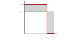
Normalized density and desired output differ, though (Fig. 1).
Subtract the two and you have the error. For a density “d,” the RMS error is:
Note that the error is a function of the input. The error is zero for a density of 0% and 100%. It is a maximum of 0.5 for a density of 50%. For an even distribution of an input signal, the average RMS error is:
So, the error is proportional to the quantization level.
By itself, the DSM output is of little use since it needs to be filtered to remove the quantization error. This can be done in several different ways. For switching power supplies, the inductor acts as a filter. For motor control, the motor’s inertia acts as the filter. For LED brightness control, the eye serves as the filter. An analog-to-digital converter (ADC), however, needs to be digitally filtered.
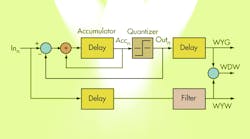
The topology in Figure 2 is used to measure the effect of a digital filter on the error. It is a DSM, built from an accumulator and a quantizer. This particular quantizer takes negative inputs and makes a reference value of –1. It also takes positive inputs and makes them a reference value of 1.
What about for an input equal to 0? Well, analog guys don’t have much need for the concept of equal. Equal is that infinitely brief moment of time when a signal switches between less than and greater than. For those not comfortable with this, we’ll just say 0 is positive. (I am sure that this will generate mail from mathematicians and engineers alike.)
The output is a combination of the input signal, delays by one sample, and the quantizer noise. The problem is that any real-world filter will distort the input. To compensate for this, the input is routed through a delay and filtered with the same type of filter used for the DSM. The DSM gives you WYG, and the separate input filter routing gives you WYW. Subtract the two to get the error (WYDW).
The filters for the spreadsheet will be sinc filters. Sometimes they are called boxcar filters or running average filters. Whatever you call them, they are just taking the average of “n” continuous samples. This filter is easy to implement in a spreadsheet and even easier to implement with digital logic, a digital signal processor (DSP), or a microcontroller. I have written several previous columns about how to implement them.2 This column is not about implementation but rather understanding what effect they have on the data.
Building The Model
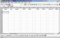
This sampled DSM will have an equally distributed, triangle-wave input with a ±1 peak-to-peak amplitude. To a reasonable measurement of the error, it will run for more than 8000 cycles. Start by opening your spreadsheet and placing the column labels in the first row (Fig. 3). I have provided a copy of the spreadsheet for those who want it, available here.
Column A is the input. It starts with a value of –1.000 in cell A3. Increment each cell below by 0.001 until you reach cell A2003. It should have a value of 1.000. Now decrement the cell below by the same amount until you get to A4002. It should have a value of –0.999. Set A4003 to:
=A3
Fill the rest of the column down to A9000. You now have input linearly distributed between ±1.
Column B includes the accumulator values for each row. Each value (accn) is a function of the previous accumulator (accn-1), the previous input (inn-1), and the previous output (outn-1). The exception is that first one (accn0) is the initial condition. In cell C3, place some initial value. In cell B3, place the following:
=B23 +A23-C2 (previous acc + previous in - previous out)
Take this entry and fill down to B9000.
Column C includes the quantized output for each row. It is a function of the accumulator value. In cell C3, place:
=IF(C3 >=0,1,-1)
The output is now one of two quantized values. Take this entry and fill down to C9000.
Column E is what you wanted (WYW). It is the input delayed by one cycle. In cell E4, place:
=A3(previous in)
Take this entry and fill down to E9000.
Column F is the filtered valued of column E. In cell F4, place:
=AVERAGE(E4:E4)
Take this entry and fill down to F9000. A filter that doesn’t average more than a single value isn’t really a filter. The number of samples length will be changed later to show how it affects the quantization value.
Column H is what you got (WYG). It is just a copy of the DSM output. In cell H4, place:
=C3
Take this entry and fill down to H9000.
Column I is the filtered valued of column H. In cell F4, place:
=AVERAGE(H4:H4)
Take this entry and fill down to I9000. The length of this filter should always match that of the filters in column F.
Column K is the difference of the two filter values. It is what you didn’t want (WYDW). The values are squared to make it easier calculate an RMD error. In cell K4, place:
=(I4 - F4)^2 (WDW)
Take this entry and fill down to K9000.
Cell L4 has the RMS error value calculated for the first 8000 error values. The cell contains:
=SQRT(AVERAGE(K4:K8003))
This calculated value is 0.816, which is the ±1 quantization level divided by the √6
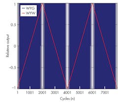
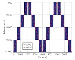
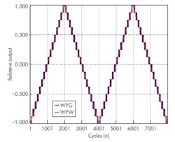
Now plot the first 8000 values of columns I and F, and you get Figure 4, which looks like a standard DSM plot. Now change both columns of filters so they average four values. Doing so will get you the plot in Figure 5, where you can see four definite levels. Also, the RMS error is now 0.204 or one-fourth the non-filtered value.
Increasing the filters to average 16 values gives you the plots in Figure 6. Again, the number of levels has increased and is proportional to the number of average samples. The RMS error is now 0.050 or one-sixteenth the non-filtered value.
The nice thing about the software model is that the resolution is proportional to the number of average samples no matter how large. With real hardware, there will be additional sources of noise that will eventually limit resolution.
Conclusion
This is a good place to stop. A digital density stream can easily be converted to a digital word. You now have a spreadsheet model that shows the effect of a simple averaging filter on the output of a DSM. Experiment a bit, and you will feel comfortable with filtering DSM in no time.
References
1. “Turn A Spreadsheet Into A Delta-Sigma Modulator,” Dave Van Ess, http://electronicdesign.com/analog/turn-spreadsheet-delta-sigma-modulator
2. Dave Van Ess, http://electronicdesign.com/author/dave-van-ess
Dave Van Ess is an application engineer, MTS, with Cypress Semiconductor. He has a BSEE from the University of Calif., Berkeley.
