Turn A Spreadsheet Into A Delta-Sigma Modulator

Pulse density modulation is just the analog portion of a delta-sigma analog-to-digital converter (ADC). It coverts an analog signal into a digital density stream. A recent online discussion about it prompted some readers to call it really cool.1 Other readers asked what the output looks like compared to its analog input.
Related Articles
- Understanding Delta-Sigma Modulators
- Using Delta-Sigma Can Be As Easy As ADC
- Lower-Power Delta-Sigma ADC Design
I tried explaining that it is a digital output stream where the average of its output equals the input value. Looking back, I am afraid I did not answer this well and figured I would try again here.
When looking at a delta-sigma modulator (DSM), you really have to look at the stream of data. Looking at just one operation is as about as useful as trying to understand Morse code with the following example:
dit
The best way to understand a DSM is to build a modulator and visually examine the output as a function of its input. I initially thought I would explain how to build one with linear components or with switched capacitor circuitry. However, this route would have required the right hardware, a signal generator for stimulus, an oscilloscope to view the output, a workbench on which to set everything up, and, of course, the spare time we all have to do it.
This file type includes high resolution graphics and schematics when applicable.
So instead I decided to make a spreadsheet model. All engineers have spreadsheets on their computer and know how to use them. The input is just a column of data, and the output is plotted. The models are straightforward to understand. It doesn’t take up any physical space, so it can be set up and used in even small moments of free time, such as between compiles. Since it looks like most any other spreadsheet you use for your job, you can work on it in the presence of a myopic, short-sighted manager who discourages any tasks other than the immediate job at hand—even if that immediate job at hand requires you to wait 10 minutes for a system build.
For those interested in hardware, I have shown many linear examples in previous columns,2 and Cypress Semiconductor has a good app note on building a switched capacitor DSM with its CY8C27x family of programmable systems-on-a-chip.3
The DSM
Figure 1 illustrates a single-bit sampled DSM. At first glance, this diagram makes it apparent why it’s called “delta sigma.” The quantized output is subtracted (delta) from the input, and the error is accumulated (sigma). This value is digitized. With negative feedback and high gain, the output attempts to match the input. Since the accumulator acts as a filter, the average of the quantized output closely matches the average of the input.
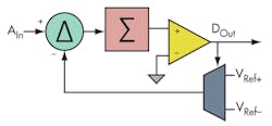
Figure 2 shows how this will be implemented.
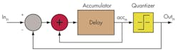
The accumulator is built from a clocked register that feeds back to itself. Here it is called delay, but it sometimes is called a register or z-1. I like the term “previous.” For this block diagram, acc is equal to the previous acc plus the previous in minus the previous out. Also, out is a function in the acc. Stated mathematically:
accn = accn–1 + inn–1 – outn–1
outn = f(accn)
You now have all the information you need to build a spreadsheet model.
Building The Model
This sampled DSM will start at 0 and continue until n is 128. I decided to make it only 128 because this was the largest value at which I could still see the distinct states of the output stream. You can always increase the sample length if you wish. Start by opening your spreadsheet and placing the column labels in the first row (Fig. 3).
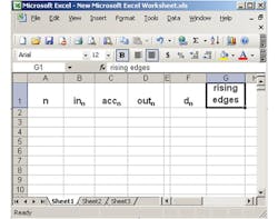
Column A includes the sample number for each row. It starts with a value of 0 in cell A3 and increments in each row ending with a value of 128 in cell A131. Column B includes the inputs for each row. It can be a function of “n” or some constant value. Start by placing a constant value of 0 in cells B3 through B131.
Column C includes the accumulator values for each row. Each value (accn) is a function of the previous accumulator (accn–1), the previous input (inn–1), and previous output (outn–1). The exception is that first one (accn0) is the initial condition. Place some initial value in cell C3. In cell C4 place:
C3+B3-D3
Or the previous acc + previous in – previous out. Take this entry and fill it in down to C131.
Column D includes the quantized output for each row. It is a function of the accumulator value. If the accumulator value is positive, the output is set to a reference value of 1. If negative, it is set to a reference value of –1. What if the accumulator value is equal to zero? Well, equal is a term analog guys don’t have much use for. I define “equal” as just that infinitely narrow moment of time going from less than to greater than (or greater than to less than). But zero is a possibility in this noise-free model, so it is defined as positive. In cell D3 place:
IF(C3 >=0,1,-1)
The output is now one of two quantized values. Take this entry and fill it down to D131.
While column D included the quantized output (–1 or 1), column F includes the digital logic value (0 or 1). This digital value would be transmitted to be digitally processed. In cell F3, place:
MAX(D3,0)
This is now a digital value. Take this entry and fill it down to F131. There is information in the frequency of this digital output, so the rising edge for each row is calculated in column G. The rising edge calculation for cell G4 is:
IF(F4 >F3,1,0)
Take this entry and fill it down to F131. In cell G2, sum all 128 of these rising edge values. You now have a DSM (Fig. 4).
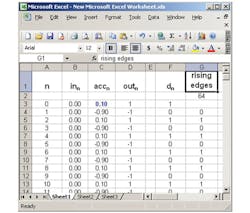
Presently this model is set with an input of zero and an initial accumulator value of 0.01. The outputs cycle between 1 and –1. This makes for a density (percentage high) value of 50%. There are 64 rising edges, which is 50% of the 128 steps. Average the 128 outputs from D4 to D131, and you get zero. (Average is just a digital filter that turns the density stream into a digital value.)
Change the initial accumulator to –0.01, and you get the same cycle and rising edge value. Change the initial value in cell C3 to 5 and notice the feedback pulls the accumulator back towards zero. Set the inputs in column B to 1.1 and verify that the DSM goes out of range. The input range for this DSM is ±1. Change the input to +0.5, and you will see that the output cycles three highs and one low (75% density), the average of the 128 outputs is 0.5, and the number of rising edges is 32 (25% of 128).
Now change the input to –0.5, and you will see the output cycles one low and three highs (25% density), the average of the 128 outputs is –0.5, and the number of rising edges remains the same at 32. The percentage of rising edges relative to the number of samples is called the output frequency and a function of the density as shown in:
fOut = min(density, 1 – density)
Now modify the inputs so B3 starts at –1 and the input in each row is incremented by 1/64. B131 with be +1. Figure 5 shows the plot.
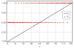
The spreadsheet provides a lot of interesting data. When the input is negative, the output stream is more lows followed by a single high. For positive inputs, the opposite is true. There are 32 of rising edges, which is the same value obtained when the input was +0.5. The average of the absolute value of this signal is 0.5.
Now change the input to make a sinusoidal output with a peak-to-peak amplitude of 1. Do this by setting B3 to:
.5*SIN(2*PI()*A3/128)
Take this entry and fill it down to B131. Figure 6 shows the plot.
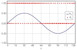
For the example, the stream still remains with single lows for positive input and single highs for negative inputs. The average of the 128 outputs is zero, and there are 44 rising edges for an fOut of 44/128 or 34.4%. The equivalent input to generate 44 inputs would be an input dc of 1/PI(). Since the average of this sinusoid rectified is, in fact, 1/p, the output frequency can be used to measure the average of an rectified signal.
This is a good place to stop. You now have a spreadsheet model of a DSM. I intend to expand on this model in my next lab—if you readers think it’s worthwhile. Until then, you have a tool that allows you to change the stimulus and view the response. Experiment a bit and you’ll feel comfortable with the DSM in no time.
References
1. “Pulse Density Modulation,” Dave Van Ess, http://electronicdesign.com/forums/ask-expert/pulse-density-modulation
2. Dave Van Ess, http://electronicdesign.com/author/dave-van-ess
3. AN2041—Understanding PSoC 1 Switched Capacitor Analog Blocks, http://www.cypress.com/?rID=2899&utm_source=TechnicalArticle-Promotions&utm_medium=DavesED-Column&utm_campaign=A-Spreadsheet-Delta-Sigma-Modulator
DAVE VAN ESS is an application engineer, MTS, with Cypress Semiconductor. He has a BSEE from the University of Calif., Berkeley.
About the Author
Dave Van Ess
Engineer
Dave Van Ess is an application engineer, MTS, with Cypress Semiconductor. He has a BSEE from the University of Calif., Berkeley.
Comment About the Article
To join the conversation, and become an exclusive member of Electronic Design, create an account today!

Leaders relevant to this article: