Practical Input-Referred Calculations in Precision Systems
Members can download this article in PDF format.
What you'll learn:
- Why input-referred calculations are valuable in gaining system insight.
- Why combining noise sources referred to input (RTI) and referred to output (RTO) is best to determine system performance.
- Defining signal gain.
- Applying LTspice and the Signal Chain Noise Analysis tool for simulation and to obtain calculations.
When designing the signal chain for an analog measurement, errors, and noise from different components in the signal chain must be tallied up and used to determine top-level performance. Specifications can be expressed fractionally as a percentage, or if they’re in linear units, they can be output-referred or input-referred. Input-referred calculations tend to cause the most confusion, but they add important insight into system performance.
Noise, Errors, and Referring to Input
Figure 1 shows a generic system block diagram for a measurement. Each block may have multiple components or stages to perform measurement functions. Every analog stage from the sensor through the analog-to-digital converter (ADC) also contributes unwanted analog noise and errors that obscure the value of the measured signal.
The data at the ADC output represents the signal combined with the total noise and error. Some of the noise and error can be reduced with calibration, compensation, and signal-processing techniques. The rest results in uncertainty in the true value of the measured quantity. For a measurement instrument, uncertainty analysis helps set key system specifications such as accuracy and precision.1,2
Referring signal-chain noise and errors to the input allows for direct comparison against the input signal. This gives insight into the overall measurement performance based on known signal characteristics and requirements. For example, calculating the total noise referred to input (RTI) sheds light on the smallest input signal that can be discerned from the noise.
Another way to think of input-referred calculation is that the data measured by the ADC is often scaled in software to represent the value of the physical quantity being measured. The original data before scaling included error and noise. Therefore, the scaled version has the same relative amount of error and noise, but it’s scaled as if it all appeared at the input along with the signal.
Combining Noise Sources RTI and RTO
For total noise calculations, noise sources need to be referred to the same place before they can be combined. While noise can be referred to other places in the signal chain, calculating the noise RTI and referred to output (RTO) is the most useful for determining system performance. The designer can choose what point in the circuit to call the input and output and what units to use.
For example, the input could be a physical quantity such as temperature in degrees Celsius, and the RTI noise can be calculated in degrees Celsius. Alternatively, the noise may be referred to the signal-chain input in electrical units like volts or amps. Similarly, the output could be defined as the data from the ADC in least-significant bits or equivalent volts, or it could be defined as the voltage at the ADC input.
An RTI noise source is a virtual noise source placed at the input that contributes the same noise in the measurement as an actual noise source. The value of each RTI noise source is determined by dividing the actual noise source by the gain from the input to that point. The noise power spectral density of the RTI noise sources is added together to determine the overall system noise spectrum.
Similarly, an RTO noise source is a virtual noise source at the output. For RTO noise, each noise source is multiplied by the gain to the output, and they’re combined at that point. If there are no noise sources after the defined output, the RTO noise matches the noise that would be measured at the output.
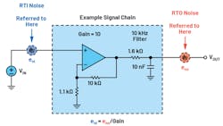
Figure 2 shows the RTI and RTO noise model for a simple signal chain that consists of a noninverting gain stage and a low-pass filter.
An imbalance exists between the two because the signal flows from input to output. RTO noise shows the noise after it has propagated through the whole signal chain, matching the total noise in the measurement. However, the RTI noise shows noise from early stages that hasn’t yet been band-limited by stages later in the signal chain.
Out-of-band noise that will be filtered out by the signal chain doesn’t affect the measured value in the end, but it does show up in the RTI noise spectrum. This isn’t technically an issue, and it doesn’t mean the RTI noise is wrong.
The RTI noise can be multiplied by the gain versus the frequency curve of the signal chain to get the RTO noise and no information is lost; however, the aim of calculating the noise RTI is to compare the noise to the input signal. By including out-of-band noise that doesn’t impact the measurement, this traditional definition of RTI doesn’t make it much easier to compare the total integrated noise against the input signal.
An Alternative Definition that Provides More Engineering Insight
The output signal can be compared to the RTO noise directly because it takes the whole signal chain into account. So, the question is: Can RTI noise be defined in a way that it can be easily compared to the input signal?
The answer reflects the real-world usage of the measurement data: Apply the same scaling to the RTO noise that would be applied to the output data in software to represent it as an input signal. Both should be calculated at the input in the same way. In other words, divide the output noise by the signal gain.
The next question is how to define the signal gain. Regardless of DC coupling or AC coupling, in most conventional linear circuits, the gain applied to the signal is flat over some bandwidth of interest by design. This bandwidth of interest can be called the signal band.
The signal has valuable information in the signal band that should be captured. The –3-dB bandwidth of the circuit is designed to be wider than the signal band to avoid dynamic errors for signals at the edges of the band. Aside from that restriction, though, the bandwidth is typically limited as much as possible to reduce noise.
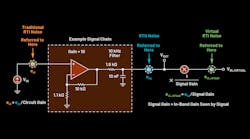
If the signal gain is defined as the gain within the signal band and that constant value is used to translate RTO noise to RTI, the RTI noise becomes more meaningful. The difference between the two models is shown in Figure 3.
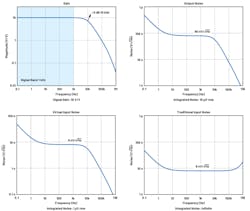
In the alternative model, RTI noise shows the noise that impacts the signal measurement, including the roll-off of out-of-band noise. Figure 4 shows the simulated differences between the two RTI methods.
The input noise curves are the same at low frequency, but they diverge when the gain rolls off. The traditional RTI noise can’t be integrated to find the total noise, whereas the virtual RTI noise can be integrated. The signal gain can be used to translate between virtual RTI noise and RTO noise for both the integrated noise and noise spectral-density values.
If the signal gain isn’t flat within the signal band, consider adjusting the signal band or modifying the circuit so that it has wider bandwidth. This helps avoid decreased performance for signals at the edge of the signal band. If that’s not possible, using the nominal gain within the signal band is most likely to match the general case and the software translation factor. However, be sure to evaluate the error and signal-to-noise ratio at the edge of the signal band to make sure they’re within performance targets.
RTI Calculations in LTspice
The versatility and accuracy of LTspice make it very useful for noise simulations. An output node and an input source are specified in the noise simulation command and output noise (RTO) is the default way to view the analysis results.
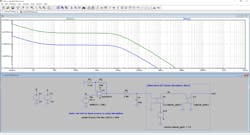
LTspice also calculates the input noise referred to the specified input source according to the traditional definition of RTI, but as demonstrated in Figure 4, integrating the traditional RTI noise doesn’t provide a meaningful result. Figure 5 shows how to add a stage to the output in LTspice so that the simulator returns the alternative virtual RTI noise.
After running the simulation, with the plot selected, add the input noise to the plot from Plot Settings—Add Trace, then choose V(inoise). This adds the input noise to the plot. The curve shape matches the output noise, which indicates that the frequency response of the whole circuit is accounted for. Press ctrl + left click on the trace title “V(inoise)” in the graph to integrate the total RTI noise.
A Web Tool for Signal-Chain Noise Analysis
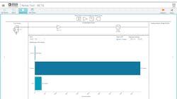
As part of the ADI Precision Studio web tools suite, the Signal Chain Noise Tool has been designed to perform noise calculations at the signal-chain level, including the integration of the total noise and the virtual RTI noise calculation (Fig. 6). Build a signal chain starting from the sensor, or start with an example, then the Signal Chain Noise Tool determines the total noise and AC performance of the full signal chain from the sensor through the ADC.
The simulation models in the Signal Chain Noise Tool use the full measured noise curves from the datasheet to provide lab-accurate results. One of the major advantages of a tool like this is to speed up the design process. The tool gives instant feedback about the effect of circuit changes on the overall noise performance, enabling faster design iterations. The completed signal chain can be exported to LTspice for custom simulations.
Conclusion
Input-referred calculations are a valuable tool to understand the expected performance of a measurement system, helping to optimize designs and inform system specifications. The virtual RTI noise method proposed here based on the measurement system architecture can be a handy modification to get more engineering insight compared with some traditional methods. Simulation tools such as the LTspice and the Signal Chain Noise Tool can aid in performing this analysis.
References
1. NIST/SEMATECH e-Handbook of Statistical Methods. NIST, April 2012.
2. “GUM: Guide to the Expression of Uncertainty in Measurement.” BIPM, 2008.
