Measuring ADC Linearity from a Sine-Wave Input
Download this article in PDF format.
What you’ll learn:
- How to measure linearity of an ADC using sine-wave input.
- How do non-idealities of a sine wave affect ADC linearity while testing it.
- Testing an ADC’s linearity.
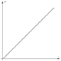
To obtain the transfer function of an analog-to-digital converter (ADC), it’s intuitive to feed a ramp signal and observe the ADC output code as shown in Figure 1. But the greater the resolution and precision of the ADC, the more complex it becomes to generate the ramp signal.
For example, let’s consider an 18-bit, 1-Msample/s ADC, where the transfer function must be measured at 1 LSB/16 = 0.0625 LSB (for hits per code = 16) precision. This means that the ramp signal should be stepped at 0.0625LSB; thus, the resolution of the ramp-signal generator should be 22 bits. However, this is severely limited by the DAC chosen for the ramp generation. And when considering the DAC’s nonlinearity, this doesn’t seem like a practical solution.
On the other hand, sine waves can be easily generated, and their purity can be worked on to meet the ADC’s performance. A sine wave of ~−120-dB total harmonic distortion (THD) contributes to an INL of ~0.26 LSB (4-V reference and 18-bit ADC). Finding an 18-bit DAC with ~0.26 LSB INL is difficult, though. Moreover, the DAC throughput would decide the linearity test time.
Thus, sine waves are the first choice for obtaining the transfer function of an ADC. Also, calculating the transfer function from sine waves isn’t as straightforward as the ramp signal, which is discussed further down.
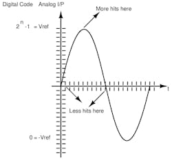
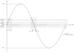
Consider a low-frequency sine wave as shown Figure 1. The frequency is so low that most of the time, the ADC consecutively captures the same code. Therefore, it can be said that most of the codes are hit more than once, or hits per code is greater than 1.
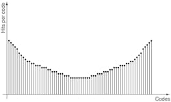
As Figure 2 shows, hits for all codes aren’t uniform. At the mid-risings, the slope of the sine wave is higher, so those codes aren’t hit as frequently. At the peaks (top and bottom peaks), the slope of the sine wave is lower, so those codes are more likely to be hit. Consequently, “hits per code” is lesser at the mid-risings and more at the top and bottom peaks.
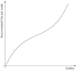
The plot of “hits per code” versus codes is as shown in Figure 3. This is famously referred to as the “bathtub” shape.
To obtain the transfer function of the ADC from the sine-wave data, let’s consider the scenario where the minimum “hits per code” is 1 from one sine-wave cycle. It’s easier to scale if we calculate for minimum “hits per code” of 1 from one sine-wave cycle. The resolution and throughput of the ADC is fixed as these are device-dependent.
The frequency of the sine wave can be varied to hit all of the codes at least once. We need to target the mid-code to be hit only once to achieve minimum hits per code equal to 1—it’s the least probable code to be hit in the entire range of codes.
We need to make sure that we hit mid-code, mid-code + 2, on the way up from 0 to Vref (Fig. 4). And on the way down from Vref to –Vref, we need to hit mid-code + 1, mid-code – 1 and so on. So, this setup would ensure that the mid-code is hit only once in the sine-wave cycle.
With the least probable code hit only once, we can be assured that all other codes are hit at least once or more than once:
The above condition ensures that the mid-code isn’t traversed again when the sine wave is rolling down from Vref to –Vref:
The first sample is the mid-code and the second sample is the (mid-code+2):
This can be simplified to:
For single-ended mode:
For differential mode:
Single-ended and differential modes have no variation as the ADC produces codes between 0 and 2n−1 irrespective of the input mode.
The number of samples to be captured is given by tin/ts:
Thus, the number of samples to capture at least one hit per code is given by the above formula. To capture (say) 32 hits per code minimum, the number of samples is 32 * (π/2) * 2n and the frequency of the sine-wave cycle has reduced 1/32 times. As a result, the frequency and number of samples are scalable with hits per code.
Let’s consider an example to get a better idea of the above calculations.
- Resolution of ADC = n = 16 bit
- Throughput of ADC = 1 MSPS, i.e., fs = 1e6, ts = 1e-6
- Hits per code = 1
The frequency of the sine wave to hit every code at least once is:
The number of samples to be captured is:
Thus, the frequency of the sine wave to be given is 9.714 Hz. This ensures that we hit all of the codes at least one time.
The linearity measurement can be more accurate with higher hits per code. Let’s now change the hits per code to 32 and recalculate the frequency of the sine wave:
- Hits per code = 32
The frequency of the sine wave to hit every code a minimum of 32 times is:
The number of samples to be captured is:
The number of samples as calculated by these equations assumes that the system is ideal. The number of samples required would usually be a bit higher than the number calculated.
Now that we have captured all of the codes from one sine-wave cycle, code width has to be calculated to obtain differential linearity (DNL) and INL. To calculate the code width, we need to calculate the transition points from the data we have. In the case of the ramp signal, the hits per each code were used to calculate the transition points. Here, too, the hits per each code can be used but the hits per each code are non-uniform in the case of sine wave unlike the case of ramp signal. Yet, the “hits per code” gives us the time difference between the transition points on a sine wave.
Consider the histogram as shown in this array:
Histogram = [h0, h1, h2, h3, h4, … h 2n−1]
where:
h0 = hits of code ‘0’
h1 = hits of code ‘1’
h2 = hits of code ‘2’
…
h2n−1 = hits of code ‘2n−1’
The transition points from 0 to 2n−1 can be traced if we use a cosine function with a phase difference of π. The cosine equation correspondingly would be cos(ωt+π), which moves from 0 to 2n−1 just as our histogram is also corresponding from codes from 0 to 2n−1.
- Transition from code ‘0’ to code ‘1’ is given by cos(ωh0ts+π)
- Transition from code ‘1’ to code ‘2’ is given by cos(ω(h0+h1)ts+π)
- Transition from code ‘2’ to code ‘3’ is given by cos(ω(h0+h1+h2)ts+π)
- Transition from code ‘3’ to code ‘4’ is given by cos(ω(h0+h1+h2+h3)ts+π) and so on
From this, the transition points of the ADC transfer function are calculated. The code width can be calculated from the difference of the transition points:
- Code width of code ‘1’ = Transition from code ‘1’ to ‘2’ – Transition from code ‘0’ to ‘1’
- Code width of code ‘2’ = Transition from code ‘2’ to ‘3’ – Transition from code ‘1’ to ‘2’
- Code width of code ‘3’ = Transition from code ‘3’ to ‘4’ – Transition from code ‘2’ to ‘3’ and so on
DNL is given as “Code width – Ideal code width.” The ideal code width is 1 LSB. The code width is being measured in LSBs; thus, DNL is also in LSB units.
The 1 LSB used in the calculation isn’t the accurate value of 1 LSB, which depends on the ADC’s reference voltage. Hence, this doesn’t involve the gain error component in the transfer function. The offset error of the ADC also doesn’t factor in the above calculations, because there’s no mapping of input voltages to output codes. Thus, the transfer function obtained from the above method doesn’t include gain error and offset error of the system.
INL is given as:
INLk = ∑DNLi , i = 0 to k for all k = 1 to 2n−1
To get the above calculations done, it’s easier if we accumulate the histogram obtained from the sine-wave data capture. Figure 5 depicts the accumulated histogram per code versus codes.
Accumulated Histogram = [ ah0, ah1, ah2, ah3, ah4, … ah2n−1]
where ahk = ∑ hi ; i = 0 to k for all k = 1 to 2n−1
- Transition from code ‘0’ to code ‘1’ is given by cos(ω.ah0.ts+π)
- Transition from code ‘1’ to code ‘2’ is given by cos(ω.ah1.ts+π)
- Transition from code ‘2’ to code ‘3’ is given by cos(ω.ah2.ts+π)
- Transition from code ‘3’ to code ‘4’ is given by cos(ω.ah3.ts+π) and so on
Until now, we have been considering one cycle of low-frequency sine wave. However, two concerns arise with this method:
- Flicker noise
- Not many sine-wave sources are good at generating a pure sine wave of such low frequencies
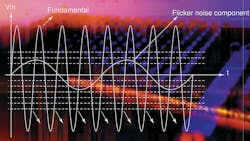
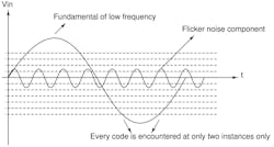
In Figure 6, we see that the presence of a lower frequency tone along with a sine wave of low-frequency fundamental can affect the histogram. Flicker noise is unavoidable in electronic systems, so there’s a need for a method that can deal with it differently.
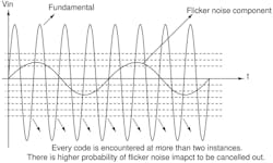
Instead of considering one sine-wave cycle, more sine-wave cycles can be used to reduce the effect of flicker noise (Fig. 7). Because the same code will likely hit in more than one sine-wave cycle with a different proportion of flicker noise at those points, the histogram of the complete dataset seems to be less affected. The hits per code can be increased to reduce the effect of noise. Therefore, having more sine-wave cycles helps us combat the disadvantages of flicker noise.
Due to inherent flicker noise in most of the electronic systems, it’s also difficult for signal generators to generate a pure sinusoidal of such low frequencies. Thus, we can break up one low-frequency sine-wave cycle into many sine-wave cycles of higher frequency. This will help us overcome the flicker noise with the same number of samples to be captured and hence the same test time.
We obtain the same histogram from one cycle of 9.714-Hz sinusoidal and 128 cycles of 1.2434-kHz (9.714 Hz * 128 = 1.2434 kHz) sinusoidal. Figure 8 shows that the effect of flicker noise can be evened out when using 128 cycles. In addition, it’s practical to obtain considerably pure sinusoidal of 1.2434-kHz frequency. (Please note that we have only depicted one flicker-noise component in the above figures for ease. In practice, there will be multiple noise components.)
Impact of Harmonics on INL Measurement
This section looks at the impact of harmonics in the input sine wave. This would show up as nonlinearity at the output of the ADC—it’s not possible to separate out the input sine-wave linearity and ADC linearity. Hence, it’s important to reduce the nonlinearity of the input sine wave as much as possible.
Also, it’s observed that the impact of harmonics on the ADC output varies with phase difference of the harmonics with respect to the fundamental. How does the phase difference of the harmonics cause different results in the linearity computation?
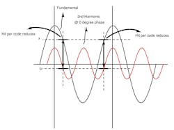
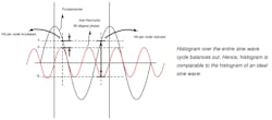
To illustrate the difference in the linearity computation, consider a second harmonic present in the input sine wave. As shown in Figure 9, the second harmonic is at a phase difference of 0° with respect to the fundamental. In Figure 10, the second harmonic is at a phase difference of 90° with respect to the fundamental.
Considering any one code ‘x’ of the sine wave, the point ‘x’ is encountered twice in a complete sine-wave cycle. When the phase difference is 0°, the point ‘x’ of the fundamental is adding on to ‘-b’ value of the second harmonic in both the encounters. This clearly means that the hit for code ‘x’ is lesser than the ideal value hit for the code ‘x’. The hit per code ‘x’ reduces because the addition of the second harmonic at that point increases the slope of the sine wave; thus, fewer samples are hit than ideal.
When the phase difference is 90°, the point ‘x’ of the fundamental is adding on to ‘a’ value of the second harmonic in the first encounter and ‘-a’ value of the second harmonic in the next encounter. As a result, the hit for the code ‘x’ is higher in the first encounter and lower in the second encounter.
Over the entire sine-wave cycle, the sample hits for the code ‘x’ balances out. This clearly occurs at all points of the sine wave, resulting in a histogram that’s equal to the histogram of an ideal sine wave without any impurities.
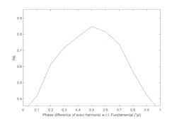
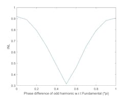
Thus, a second harmonic at a phase difference of 90° with respect to the fundamental in the input sine wave doesn’t contribute to the ADC linearity in the measurement. On the other hand, a second harmonic at a phase difference of 0° with respect to the fundamental in the input sine wave is the biggest contributor to the ADC linearity. This can be observed for all even harmonics—even harmonics at a phase difference of 90° don’t contribute to the ADC’s linearity. On the contrary, it’s true that odd harmonics at a phase difference of 0° don’t contribute to the ADC’s linearity.
Figure 11 depicts the variation of INL with respect to the phase difference of even harmonics with respect to the fundamental.
Figure 12 reveals the variation of INL with respect to the phase difference of odd harmonics with respect to the fundamental.
This means that the presence of even harmonics at 0° and odd harmonics at 90° phase with respect to the fundamental doesn’t affect the measurement of INL. Since the harmonics aren’t intentional in the signal, it’s difficult and impractical to control the phase difference of the harmonics. Only the accurate knowledge of all harmonics and their phase with respect to the fundamental would enable us to obtain the ADC linearity separately from the signal-chain linearity.
Chandana Krishna is an Analog Engineer at Texas Instruments.
About the Author
Chandana Krishna
Analog Engineer, Texas Instruments
Voice Your Opinion!
To join the conversation, and become an exclusive member of Electronic Design, create an account today!

Leaders relevant to this article:
