Modeling on Mondays: SPICE Modeling of Common Active Devices—An Overview (Part 1)
What you’ll learn:
- A variety of linear models are available to represent common active electronic devices such as transistors and vacuum tubes.
- Devices operating under large-signal conditions often require nonlinear models.
- Transistors can have crazy device to device variations, whereas vacuum tubes are relatively uniformly produced.
Welcome to the first of Electronic Design’s multipart Modeling on Mondays series, where experts share their knowledge about SPICE modeling methodology and applications. Please send an email to our mostly-Analog editor, AndyT, if you’d like to propose contributing to this series, or other analog topics, by writing for our readers. Feel free to leave your thoughts and experiences in the comments, below.
Introduction
As we go about analyzing (or synthesizing or designing) systems, our quest is for methods that make analysis easy―or, at least, tractable―for us. In most cases, we would love to have the system we’re analyzing be, if not truly linear, “close enough” to linear for all practical purposes. Why? Because there’s a vast array of analytical methods that are generally applicable to such systems.
If a system can’t be imagined to be linear to within a reasonable degree of accuracy, then next in order of attractiveness would be the assumption that the system is piecewise-linear. Analysis of piecewise-linear systems is just a little bit more involved than that of linear systems.
If the device, circuit, or system defies being modeled accurately as linear or piecewise-linear, then we must deal with the nonlinearities as best as possible. No general methods are available for the analysis of nonlinear systems.
Common active electronic devices, whether solid-state or “hollow-state” (i.e., thermionic “tubes,” “valves”), are wildly nonlinear. But we can take approaches that help us get through the task of carrying out, with reasonably accurate results, an initial analysis of a circuit that employs such devices.
Each active device in the signal path within a circuit presents a connecting relationship between the portion of the circuit controlled by the device and the portion of the circuit controlling the device. It’s this generally nonlinear connecting relationship that we must deal with, which may be described by one of the following:
- A transfer relation obtained graphically by observing, along an appropriate path (such as a load line), the family of output curves for the device.
- A nonlinear governing equation or approximation.
- A linear approximation to the actual nonlinear governing equation.
We note that most electronic amplifiers and oscillators are designed with the intention that the active devices in the signal paths operate within, or at the boundaries of, their active regions. Such restrictions on an active device's operation typically result in the nonlinearity observed being less “ugly” than if the region of operation for the device was unrestricted.
Models for Active Devices Under DC Conditions
Generally, the first order of business in analyzing an electronic circuit is to determine particular voltages and currents at quiescence. That is, we want to analyze the circuit under DC conditions without an input signal present.
If the device involved is a field-effect transistor (FET) (JFET, MOSFET, CNTFET, etc.), an approximation to the nonlinear governing equation relating vGS, iD, and vDS is typically used. If the device is a bipolar junction transistor (BJT), often a linear approximation to the iC vs. iB relation is used. If the device is a vacuum tube (“VT”), graphical means are most often employed to obtain the transfer relation, although circuit simulators such as SPICE can be useful once a sophisticated compact model is developed for the device.
For many active devices, the values of parameters used in describing their operation are very poorly controlled during their manufacture. For example, the pinchoff voltage and saturation current for a FET might vary over a 10-to-1 range within type. The forward current gain for specimens within the same type of BJT might vary over a 3-to-1 or 4-to-1 range. Variations in values of parameters for VTs will generally be significantly smaller; a 20% variation might be typical for tubes coming off a well-controlled manufacturing line.
Thus, it might be meaningful to plot a typical family of curves for a VT, but a “typical” family of curves for a FET or BJT would generally provide little meaning. However, if the measured curves for the particular specimen of the active device used in the circuit being analyzed were known, then a plot of that family of curves would, of course, be very informative to the analysis.
Models for Active Devices Under AC Conditions
When we set about analyzing a circuit under AC, or dynamic, signal conditions, we usually start out with the assumption that the circuit is operating under small-signal conditions; i.e., we assume that every quantity (voltage or current) of interest varies only “a little” from its quiescent value. In effect, we do a Taylor-series expansion of the variable of interest about its quiescent point and truncate the expansion after the linear term.
The incremental change in the quantity of interest is its AC component, and we have described it by a linear relationship. Thus, with this small-signal approximation describing the active device under AC conditions, we can use linear-circuit-analysis techniques to analyze the overall circuit under AC conditions (given that the rest of the circuit is described by linear circuit elements only).
A number of linear models can be readily applied to the active device involved.
Two-Port Parametric Models
One set of models is the six parametric models relating the terminal voltages and currents of a linear two-port network having no internal independent sources. Such models are described in any good introductory text on circuit theory and include the open-circuit impedance (z-parameter), the short-circuit admittance (y-parameter), the transmission (a-parameter, or ABCD), the inverse transmission (b-parameter, or A'B'C'D'), the hybrid (h-parameter), and the inverse hybrid (g-parameter) models.
Of those, only the h-parameter and y-parameter models receive much use in describing active electronic devices. The typical use for the h-parameter model is to describe BJTs at low frequencies. The y-parameter model finds use in describing BJTs and FETs at higher frequencies (typically, at 10 MHz and above). The z-parameter model, although used on occasion in the “early days” to model junction transistors, isn’t generally used nowadays to describe active devices. However, it is often used to model linear amplifiers.
Equivalent Circuits Based on Ideal, Linear Circuit Elements
Another class of linear models uses ideal, linear, lumped-parameter circuit elements (ideal resistors, capacitors, inductors, and dependent sources) to characterize active devices in terms of their device parameters. Some of these models can become very involved, particularly as the modeler attempts to achieve increasingly wideband representations of the active device under consideration.
Although the more complex models are very useful when handed over to a circuit-analysis-and-simulation program such as SPICE, the models of intermediate complexity are useful in “hand” calculations.
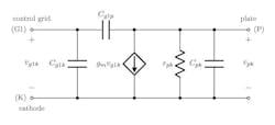
The gm equivalent circuit (or model) for vacuum tubes. The so-called gm equivalent circuit (Fig. 1) is a very useful model for a VT operating at frequencies of up to several megahertz.
A model similar in structure is suitable in representing FETs.
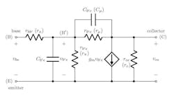
The hybrid-π equivalent circuit for transistors. The hybrid-π model (Fig. 2) is a Π-type equivalent circuit developed in the early 1950s to yield a model for the transistor similar in form to the gm model for the vacuum tube. In some senses, it’s a modification of the Early equivalent circuit and Angell’s bridged-T equivalent circuit, which grew out of Early’s model.
The hybrid-π model works well at frequencies of up to about ωα/2, where ωα is the so-called α-cutoff frequency of the transistor. Another advantage of this model, besides its similarity to the gm model, is that the gain of the dependent source, as well as all resistances and capacitances within the model, are, to a first approximation, frequency-independent.
Generalized equivalent circuit for active devices. From Figures 1 and 2, it seems possible that a generalized equivalent circuit for active devices could be developed. There are some advantages to doing so, a major one being that a single, general analysis of a linear circuit, independent of the active device chosen, can be performed.
Scattering-Parameter Model
In addition to the aforementioned six parametric models based on terminal voltages and currents, there’s the “S-parameter model” that’s based on incident and reflected energy at the various ports of the device or network under consideration.
S-parameters are particularly useful in representing devices and networks at ultra-high and microwave frequencies. Given a set of S-parameters, the corresponding set of parameters associated with any of the other models mentioned above can be calculated. An automated laboratory instrument called a network analyzer, coupled with an S-parameter test set, makes the work of characterizing a device or network over a frequency range of a few hundred megahertz to tens of gigahertz a relatively easy task.
In the analysis of circuits at frequencies in the megahertz region and below, it’s generally typical to only use h-parameter, y-parameter, gm, and hybrid-π models—and those models could be further simplified whenever warranted. At low frequencies (roughly 100 kHz and below), all of these models are very simple, as is the conversion among them.
When studying the datasheets from a variety of manufacturers for various active devices, it will become apparent that there’s no real consistency in the presentation of small-signal parameters, even by a given manufacturer for a particular class of device (e.g., BJTs). Any of a set of characteristic output curves, a list of typical values of h or y parameters at a given frequency, a graph of typical values of h or y parameters (both real and imaginary parts) over a range of frequencies, or typical values for some of the hybrid-π parameters can be presented.
Without setting up equipment and making measurements on a statistically significant number of the active devices to be used, experience is invaluable in interpreting the information gaps left by the datasheet.
Large-Signal Models
This, the first of an Electronic Design multipart series on active device modeling and simulation, mentioned several linear models that are useful in describing various active devices under small-signal conditions. If the circuit is being considered under large-signal conditions, the nonlinear nature of the active device makes itself evident in operation. Any careful analysis of the circuit under such conditions requires, in general, either graphical techniques or a numerical approach.
About the Author
Stephen A. "Jack" Dyer
Professor Emeritus of Electrical and Computer Engineering, Kansas State University
Jack Dyer is Professor Emeritus of Electrical and Computer Engineering, Kansas State University. He holds degrees in physics, electrical engineering, and engineering, and he spent most of his career as a faculty member, having taught over 80 different courses in mathematics, physics, electrical and computer engineering, entrepreneurship, and music. Jack’s research was broadly in digital communication systems, digital signal processing, instrumentation and measurement, spectrometry, and numerical methods, but his fun has been in analog electronics. His consulting practice centered largely on engineering forensics and assistance in product design.
When not resto-modding a Hammond or an attendant Leslie speaker system, he’s either playing in a band or searching for opportunities to bore holes in the sky via helicopter, gyroplane, or fixed-wing aircraft.
Voice Your Opinion!
To join the conversation, and become an exclusive member of Electronic Design, create an account today!

Leaders relevant to this article:
